This paper is made available online in accordance with publisher policies. Please scroll down to view the document itself. Please refer to the repository record for this item and our policy information available from the repository home page for further information.
To see the final version of this paper please visit the publisher’s website. Access to the published version may require a subscription.
Author(s): Yong Cai and Christos Mias
Article Title: Application of multisection recursive convolution in 3D FETD-FABC simulations
Year of publication: 2008 Link to published article:
http://dx.doi.org/10.1002/mop.23455
For Peer Review
Application of multi-section recursive convolution in 3D FETD-FABC simulations
Journal: Microwave and Optical Technology Letters
Manuscript ID: MOP-07-1259
Wiley - Manuscript type: Research Article
Date Submitted by the
Author: 16-Oct-2007
Complete List of Authors: Cai, Yong; Warwick University, Engineering Mias, Christos; Warwick University, Engineering
For Peer Review
Application of multi-section recursive convolution in 3D FETD-FABC
simulations
Yong Cai and Christos Mias
ABSTRACT: The multi-section recursive convolution (MS-RC) methodology is successfully applied to the Finite Element Time Domain Floquet Absorbing Boundary Condition modelling of doubly periodic structures. It is shown that late time instability can be delayed by improving the accuracy of RC and it can be effectively avoided by employing extrapolation.
Key words:time domain, finite element method, recursive convolution, periodic structures
Corresponding author: Yong Cai
Corresponding author’s email: e-mail: [email protected]
Affiliation:
Applied Electromagnetics and High-Frequency Telecommunications Laboratory, Communications and Signal Processing Group, School of Engineering, University of Warwick, Coventry CV4 7AL, U.K. Emails: [email protected] and [email protected]. 1
For Peer Review
1. INTRODUCTION
The finite element time domain (FETD) method was employed recently to model plane wave scattering from 3D doubly periodic structures [1]. Emphasis was given to the accurate Floquet Absorbing Boundary Condition (FABC) [1]. But, although accurate, the FETD-FABC method suffers from the presence of time consuming convolution integrals. Very recently, a recursive convolution (RC) [2] methodology, henceforth called the multi-section RC (MS-RC) has successfully been employed to reduce considerably the time requirements of the 2D scalar FETD-FABC [3]. This success encouraged us to investigate the application of MS-RC to the 3D vector FETD-FABC modelling of periodic structures knowing that the accuracy of the computation of the FABC affects stability [1].
In this paper, we demonstrate that the MS-RC methodology of [3] can be applied successfully to the modelling of plane wave scattering from a 3D doubly periodic structure. The late-time field growth observed, which we henceforth term as late time instability, is delayed by improving the accuracy of the exponential summations needed in the MS-RC and by employing temporal triangular basis functions [1] to improve the accuracy of the numerical evaluation of the single-time-step integral terms present in the MS-RC. In addition, the matrix-pencil extrapolation method [4] is employed to effectively avoid the late time instability that is present in 3D vector FETD simulations [5, 6] without stability correction schemes. The numerical results presented show that the 3D MS-RC-FETD-FABC code is 3 times faster than the 3D FETD-FABC employing standard convolution.
2. FETD-FABC FORMULATION
In our 3D formulation, the vector electric field is used as the working variable. Since Floquet’s theorem applies in an infinite doubly periodic structure, only a single unit cell needs to be analysed (Figure 1). In the frequency domain, where the time harmonic term ej t is suppressed, 1
For Peer Review
the theorem can be expressed as( )
r E( )
r rE ; = ; jk0•
p e (1)
Ep is the periodic part of the electric field, r= xxˆ + yyˆ +zzˆ , k0= /c is the wavenumber in
free space, c is the speed of light in free space and is a vector whose coefficients are determined by the direction of the incident plane wave, i.e.
y x
y
xˆ yˆ sin inccos incˆ sin incsin incˆ
x + = +
= (2)
inc
and inc are defined in Figure 1.
The Galerkin weighted residual method is employed to solve the vector wave equation [7]. The weighting function is assumed to be of the form [7]
( )
r W( )
r rW = +jk0 •
p e (3)
Wp is the periodic part of the weighting function. Hence, the following frequency domain Galerkin weighted residual formulation in terms of the periodic part of E and W can be derived
(
) (
)
[
]
(
)
(
) (
) (
) (
)
[
]
(
)(
)
(
)
•(
)
µ + •
µ =
• •
µ ×
• × ×
• × µ +
• µ
× • × µ
2
1 , 0 ,
, ,
, 0 , ,
,
2 0 0
2 2
0
1 1
1 1
sin 1
S t pz pz
t p t p r
S t pz pz
t p t p r
V p p
r
V p p p p
r
V p p
r inc
r
V p p
r
dS E jk E z
dS E jk E z
dV k
dV jk
dV k
dV
E W
E W
E W
W E
E W
E W E
W
(4)
where µr and r are the relative permeability and relative permittivity respectively.
y x
Wp,t =Wp,xˆ+Wp,yˆ . Ep,t =Ep,xxˆ+Ep,yyˆ and Ep,z are the tangential and normal
components, respectively, of the periodic part of the total field with respect to surfaces S1 or
S2. A similar notation is used for the incident field, E E , , zˆ
inc z p inc
t p inc
p = +E . S1, S2 and V are defined
in Figure 1. In the formulations and simulations that follow S1 is assumed to be at z=z1=0. The
symbol t = xxˆ+ yyˆ denotes the tangential gradient operator. The surface integrals
For Peer Review
along periodic boundary pairs (Sx and Sy, see Figure 1) cancel out each other due to the
periodic boundary conditions and the fact that the normal unit vectors of the boundaries have opposite directions. Note that the FEM meshes at the boundaries of each periodic boundary pair are identical. At the non-periodic boundaries S1 and S2 the Floquet ABC is derived using
the Floquet harmonic expansion [7] and the orthogonality property of these harmonics. When this boundary condition is employed in (4) and equation (4) is transformed to the time-domain via the inverse Laplace transform (ILT), the following time-domain weighted residual equation is obtained
(
) (
)
[
]
(
)
(
)
(
)
) ( ) ( ) ( 1 1 1 1 sin 1 1 2 1 2 2 2 2 2 2 2 t t t F dV t c dV t t c dV t c dV S V p p r V p p p P r V p p r inc rV p p
r = • • µ + × • × × • × µ + • µ + × • × µ E W E W E W E W E W (5) where
( )
( )
• • + • = dt t d dS c dt t d dS c t F inc t pS pt
inc inc
t p
S pt
inc S , , , , 1 1 cos 2 cos 2 )
( W E W E (6)
( )
( )
( )
( )
( )
( )
! ! = ! ! = • + • • + • ! ! = ! ! = • + • ! ! = ! ! = • + • ! ! = ! ! = • + • " + " + " + " + " • = m n S j x p mn S j y p S j y p mn S j x p
m n S
j y p mn S j y p
m n S
j x p mn S j x p
m n S
j t p mn S j t p dS e t E t dS e W dS e t E t dS e W dS e t E t dS e W dS e t E t dS e W dS e t t dS e t mn t mn t mn t mn t mn t mn t mn t mn t mn t mn t 2 , 1 , 2 , 1 , 2 , 1 , 2 , 1 , 2 , 1 , 2 , 1 , 2 , 1 , 2 , 1 , 2 , 1 , 2 , 1 , ) ( * ) ( * ) ( * ) ( * ) ( * , ) 4 ( , , ) 4 ( , , ) 3 ( , , ) 2 ( , , ) 1 ( , 2 , 1 r r r r r r r r r r E W (7)
The symbol ‘*’ denotes the convolution operator. The symbols m,n, are the Floquet harmonic
indices. In the computations, the m,n summations are finite, i.e. –MF#m#MF and
–NF # n #NF. Furthermore,
For Peer Review
y xy
xˆ , ˆ 2 ˆ 2 ˆ
, y x n y m x t,mn D n D m $ + $ = % + % = (8)
where Dx and Dy are the periods (Figure 1).
In (7), the time functions " are of the following form
( )
( )
t C( ) ( )
{
C f( )
t C( )
f( )
t C( )
f( )
t C( )
( )
t jC( )
q( )
t}
mn q mn q mn q mn mn q mn q qmn = + + + () + (
" 0 1, 1, 2, 2, 3 3, 4 5, (9)
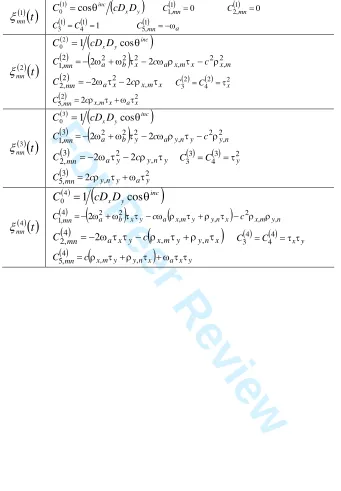
where (( )t and ( )( )t are the Dirac delta function and its first order time derivative respectively. The time-independent coefficients C are given in Table 1. The three time functions in (9) are
( )
t e J(
t)
f mn = j at ab
0 ,
1 , f
( )
t j e J(
abt)
t j ab
mn = a 1
,
2 ,
( )
(
)
t t J e t f ab ab t j abmn = 2 a 1
, 3 (10) where 2 2 b a
ab= + , a inc
(
tmn)
c
, 2
cos •
= , 2 , 2
2 2
cos inc tmn
b
c
= (11)
( )
* 0J and J1
( )
* are the zero and first order, respectively, Bessel functions of the first kind [8]. Six degree of freedom (d.o.f.) tetrahedral edge elements are employed in the FE discretisation of the unit cell [9]. For the surface integrals, three d.o.f. triangular edge elements are employed. Within each triangular element, Ep is expressed as(
x y t)
( )
x yEp j( )
tj j p , 3 1 , ; , = = N E (12)
Ep,j(t) is a d.o.f and N are the vector basis functions [9]. From (9) and (12) it follows that the convolution "( )mnq
( )
t +Ep,j( )
t in (7) can be expressed as( )
( )
( )
( ) ( )( )
( )
( )( )
( )
( )( )
( )
( )[
( )
]
( )( )
, -, . / , 0 , 1 2 + + + + + + + = + " t E jC dt t E d C t E t f C t E t f C t E t f C C t E t j p q mn j p q j p mn q j p mn q mn j p mn q mn q j p q mn , , 5 , 4 , , 3 3 , , 2 , 2 , , 1 , 1 0 , (13)For Peer Review
3. MULTI-SECTION RC FORMULATION
The derivation of the MS-RC formula is described in the 2D scalar FETD-FABC work of reference [3]. Hence, in the present 3D vector MS-RC-FETD-FABC research we focus on the exponential summation approximation of the 3 functions present in the 3D formulation and our attempts to improve the accuracy of these approximations. For convenience, let = abt.
Hence, the three time functions J0( abt), J1( abt) and J1( abt)/( abt) in (10) are re-written as
( )
3 =( )
341 J0 , 42
( )
3 =J1( )
3 , 43( )
3 =J1( )
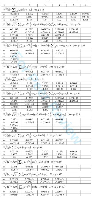
3 3 (14)In this work we choose to divide the ‘time’ range of into four sections: 0# 3 #18, 18 <3 #50, 50 <3 #335 and 335 <3 #2×10⁴. In each section, the MATLAB curve fitting toolbox is employed to approximate the time functions (14) with exponential or sinusoidal terms (Table 2). The number of sections is chosen using a trial and error approach in which the number of the sections is increased until a sufficiently large time window of practical stability is obtained in the MS-RC-FETD-FABC simulations. For the first section, of each function, MATLAB is used to approximate directly the functions in (14) using sinusoidal terms (Table 2). However, for sections 2, 3 and 4 use is made of the large argument approximation [8]
( )
3 5 $( )
3 3 $ $4 2 cos
2 12 k
Jk (15)
Hence, using exponential terms, MATLAB is used to approximate the function -1/2 for 41( ),
42( ), and the function -3/2 for 43( ) rather than the functions (14) themselves.
We tried to improve the accuracy of the above approximations since such improvement
results in a more accurate RC and delays the onset of late time instability (see the numerical
results section). Thus, the MATLAB approximation in the second and third argument sections
(18 <3 #50 and 50 <3 #335) can be improved, heuristically, by adjusting the phase term in
the cosine function in (15). In addition, to further improve the accuracy of the approximation,
the curve fitting error [3] of the functions 1/2, 3/2 was fitted by a summation of sinusoidal
For Peer Review
functions and this summation was added to the original summation. For example, the improved approximation for the function 42( ) in its third section, as shown in Table 2, is
( )
( )
(
)
(
)
=
= 3 3 $ + 3+
$ = 3 4 1 1 4 1 3
2 2 cos 2.99 4 sin
~
i i i i
i h
ie i a b c (16)
whereas prior to these improvements it was
( )
( )
[
]
(
)
4 3 cos 2 ~ 4 1 32 3 = $ 6 3 $
4 = 3
i h i
i
e (17)
The curve fitting absolute error [3] over the argument region 0# 3 #2×10⁴, for each of the
approximations to 41( ), 42( ) and 43( ), is plotted in Figure 2. In Figure 2(d) we compare the
errors of the summations in (16) and (17) over the range 50 <3 #335. Note that the
coefficients in Table 2 are generic as they are the same for all harmonics (m, n) and for other
periodic structures.
Based on Table 2, the time functions f1,mn(t), f2,mn(t) and f3,mn(t) in (9), in any section g, can
be expressed as a summation of exponential terms. For example, f1,mn(t) is approximated as
( )
( )
( )( )
( ) ( ) ==
5 g ab
g i Q i t B g i g mn g
mn t f t A e
f , 1 , 1 1 , 1 , 1 , 1 ~ (18)
where Q1,g denotes the total number of exponential terms. Consequently, at the current time
step M (t=M7t), R1M = f1,mn
( )
t +Ep,j( )
t is approximated as( )
( )
]
( ) ( ) ( )( )
]
( ) ( )]
( ) ( ){
}
{
( )]
( )}
( ) ( )]
( ) ( ) ( ) ( ) ( ) ( )]
( ){
}
( )= 7 7 = = 7 7 7 = 7 = = 7 7 7 7 7 = 7 + 8 + , , -,, . / , , 0 ,, 1 2 7 7 + 8 = 8 + 8 = + = G G G G ab G i g g g g g g g ab g i G G g g g G g g Q i j p N M N M G mn t N M M G i t B G g j p N M N M g mn j p N M N M g mn Q i t N M t N M M g i t B Q i t N M M G i G g Q i t N M t N M M g i t N M M G t N M t N M G g M g M d E t M f e d E t M f d E t M f e R R R , 1 1 1 1 , 1 1 1 , 1 1 , 1 , 1 , 1 1 1 1 1 ,
1 1,
1 0 1 , , 1 1 1 , 1 1,
,
1 1,
For Peer Review
The symbols of (19) are defined in [3]. Here G=4. For consistency, we replace some symbols of equation 21 in [3], e.g. ‘ ’ is replaced by ‘mn’, ‘9p’ by ‘Ep,j’, ‘ c ’ by ‘ ab’. The subscript ‘1’ in R denotes the RC for the function f1,mn(t). Similar expressions hold for the
other convolution terms in (13). Equation (19) is the formulation step prior to equation 21 in [3]. Equation 21 in [3] is obtained if the single-time-step integral terms in (19) are discretised using trapezoidal integration.
In this paper, we interpolate the electric field variable in the integral terms of (19) using temporal triangular basis functions. For example, over the time interval (M–1–Ng) t # t # (M–Ng) t, Ep,j(t) can be approximated as
( )
[
t(
M N)
t]
t E E E t E g N M j p N M j p N M j p j p g g g 7 7 + 5 1 1 , , 1 , , (20)
and therefore using (18) and (20) the integral term with limits (M–1–Ng) t#t# (M–Ng) t in (19) is analytically evaluated as
( )
(
)
( ) ( )( )
( ) ( ) ( )(
)
( ) ( )[
]
( )(
)
( )[
]
= 7 7 7 7 7,-,
.
/
,0
,
1
2
+
7
+
7
7
=
7
g g ab g i g ab g i ab g i g g g Qi M N
j p t B ab g i N M j p ab g i t B ab g i t B N g i j p t N M t N M g mn
E
e
t
B
E
t
B
e
t
B
e
A
d
E
t
M
f
, 11 , 1
, 2
,
1 1,
1
1
1
~
(21)
A similar approach can be followed to evaluate analytically the other integral terms.
4. NUMERICAL RESULTS
To numerically examine the proposed MS-RC-FETD-FABC formulation, we consider the frequency selective surface (FSS) example of [1] (Figure 1). The unit cell consists of a perfectly electrically conducting patch (Lx= 2.5mm, Ly=5mm) embedded symmetrically in a dielectric slab of thickness h=2mm. The periods are Dx=Dy=10mm. The distance between the non-periodic finite element boundaries (S1 and S2) and the closest parallel dielectric slab
surface is da=8mm. The slab’s relative permittivity and relative permeability are r=2 and µr=1
For Peer Review
respectively. The angles of plane wave incidence are inc=30º and inc=0º and the incident electric field vector is along the y-direction. The time-domain waveform of the incident field is a sinusoidal wave modulated by Gaussian pulse with parameters = 400 t, = 100 t, and fc= 15 GHz. These parameters are defined in [3]. Furthermore, the time step size is 7t= 0.3ps and the number of harmonics is restricted to MF=NF=2.
Transient responses of the electric field d.o.f. Ep,j(t), associated with a surface element edge on boundary S1, are shown in Figure 3. Two of these transient responses correspond to
simulations employing the summation approximations (16) and (17). In both simulations, the triangular basis function is employed. The approximation of (16), being more accurate, delays the onset of late-time instability. For comparison purposes, Figure 3 also shows the transient response when the less accurate trapezoidal integration is employed in the RC. The results confirm the advantage of using the triangular basis function in RC computations and confirm the remark in [1] that the accuracy of convolution affects stability.
In Figure 4, the transient response of Atot
( )
z ty 1; is plotted. A
( )
z ttot
y 1; is the y-component of
( )
z ttot t 1;
A defined as
dS
t
z
y
x
D
D
t
z
A
t
z
A
t
z
S pt y
x tot
y tot
x tot
t
=
+
=
1
)
;
,
,
(
1
ˆ
)
;
(
ˆ
)
;
(
)
;
(
1 1x
1y
E
, 1A
(22)By comparing the results of Figure 4 with those of Figure 3, it can be deduced that the transient
response of the fundamental harmonic coefficient is stable over a longer time interval despite
the fact that during this interval there is an unstable field growth. This observation agrees with
the relevant statement made in [6]. Figure 4 also emphasises the stability benefit arising from
the use of temporal triangular basis functions.
To avoid the growing effects of late time instability and speed up the simulation of highly
resonant structures, extrapolation is used. In this paper extrapolation is based on the
For Peer Review
matrix-pencil method [4]. The matrix-pencil software employed was based on equations (1-15) of [4]. The extrapolation of the Atoty
( )
z1;t component is based on the transient timeinterval 60007t#t#72007t obtained using triangular basis functions. For the Axtot
( )
z1;tcomponent extrapolation is based on the time interval 30007t#t#42007t. These intervals are well within the region of stable results for the field values. The incident wave has already died out prior to these intervals. The accuracy of the extrapolated data is demonstrated by comparison with the actual data in Figure 5.
The accuracy of the developed MS-RC-FETD-FABC code is examined in Figure 6 where the normalised power of the reflected (m,n)=(0,0) fundamental harmonic, defined as
( )
(
)
(
)
(
)
21 , 1
,
2 1 , 1
, 1
1
ˆ ) ; ( ;
ˆ ) ; ( ;
ˆ ) ; ( ;
1 E z
z E
z A
+ +
=
z E z
z E z
z A z
P
inc z p inc
t p
inc z p inc
t p tot
z tot
t
z ref
(23)
is plotted against frequency. The discrete Fourier transform (DFT) is applied to (22) to obtain
(
z1;)
tot tA . The normal component, Atotz (z1; ) is then obtained using •( 0E) = 0. The
MS-RC-FETD-FABC results with extrapolation (using 36000 time steps) and without extrapolation (using 7200 time steps) are compared with the FETD results in [1] and the CST Studio Suite 2006 frequency-domain solver results [10]. The good agreement between all the results suggests that the MS-RC proposed in [3] can be employed in the FETD-FABC simulation of doubly periodic structures. The slight shift between our results and those of [1] and CST is not due to the MS-RC but to the spatial discretisation accuracy i.e. more accurate results are expected if the mesh is refined and higher order elements are employed.
To examine the computation time requirements of the proposed MS-RC-FETD-FABC we considered a 5000 time step simulation without extrapolation. The required time was 89min. When compared to the 273min required by the FETD-FABC employing a standard 1
For Peer Review
convolution, the MS-RC-FETD-FABC code is 3 times faster. Our simulation times correspond to the time marching part of the simulation, i.e. they ignore the time of assembly and inversion of the FEM matrix at the start of the simulation.
5. CONCLUSION
It is demonstrated that the MS-RC methodology proposed in [3] can be applied to the FETD Floquet ABC simulation of 3D doubly periodic structures resulting in a significant reduction of computation time compared to FETD-FABC formulations where the convolution is computed in a standard fashion. It is also demonstrated that using extrapolation practically avoids the effect of late time instability which is always present in 3D vector FETD simulations when no stability correction scheme is applied. To improve further the stability of our results, we shall focus our future research on bettering the RC methodology through improved exponential summation approximations.
ACKNOWLEDGMENTS
We acknowledge the use of Fortran FEM subroutines written by Tian H. Loh and the use of the Harwell Subroutine Library, Harwell Laboratory, Oxfordshire, UK. This work was supported in part by a Dorothy Hodgkin Postgraduate Award (EPSRC/Hutchison Whampoa). 1
For Peer Review
REFERENCES
1 L. E. R. Petersson and J. M. Jin, Analysis of periodic structures via a time-domain finite-element formulation with a Floquet ABC, IEEE Trans Antennas Propag 54 (2006), 933-944.
2 Semlyen and A. Dabuleanu, Fast and accurate switching transient calculations on transmission lines with ground return using recursive convolutions, IEEE Trans Power App Syst 94 (1975), 561–571.
3 Y. Cai, and C. Mias, Fast Finite Element Time Domain – Floquet Absorbing Boundary Condition modelling of periodic structures using recursive convolution, IEEE Trans Antennas Propag 55 (2007), 2550-2558.
4 R. S. Adve, T. K. Sarkar, O. M. C. Pereira-Filho, and S. M. Rao, Extrapolation of Time-domain responses from three-dimensional conducting objects utilizing the matrix pencil technique, IEEE Trans Antennas Propag 45 (1997), 147-156.
5 C.-T. Hwang, and R.-B. Wu, Treating late-time instability of hybrid finite-element/finite-difference time-domain method, IEEE Trans Antennas Propag 47 (1999), 227-232.
6 D.-K. Sun, J.-F. Lee and Z. Cendes, The Transfinite-Element Time-Domain Method, IEEE Trans Microwave Theory Tech 51 (2003), 2097-2105.
7 R. L. Ferrari, Spatially Periodic Structures, Chapter 2 in Finite Element Software for Microwave Engineering, Eds. T. Itoh, G. Pelosi and P. P. Silvester, Wiley, New York, 1996. 8 M. Abramowitz and I. A. Stegun (Eds), Chapter 9.2 in Handbook of Mathematical Functions
with Formulas, Graphs, and Mathematical Tables, 10th printing, 1972.
9 J. M. Jin, The finite element method in electromagnetics, Wiley-IEEE press, New York, 2002. 10 CST, Computer Simulation Technology, Darmstadt, Germany, www.cst.com.
For Peer Review
Figure captions
Figure 1 Unit cell of a doubly periodic structure. The incident angle is defined by inc and inc. The Dx and Dy are the periods along the x and y directions.
Figure 2 The absolute error of the exponential summation approximation of the functions: (a) J0( ); (b) J1( ); (c) J1( )/ ; (d) black line (16), gray line (17).
Figure 3 The transient response of Ep,j(t) on the surface S1. Dashed line: trapezoidal
integration; dotted line: result using temporal triangular basis function with 4( )3
( )
32
~ given by
(17); solid line: result using temporal triangular basis function with 4( )3
( )
3 2~ given by (16).
Figure 4 Transient response of Atoty (z1;t). Dotted line: trapezoidal integration approach (6858 time steps are shown); solid line: temporal triangular basis function (13894 time steps are shown). The inset is a magnified version of the time interval within the dashed rectangle.
Figure 5Comparison of extrapolated and actual transient results forAtoty (z1;t). Dotted line: actual data; solid line: extrapolated data.
Figure 6 The normalised power carried by the reflected (m,n)=(0,0) fundamental Floquet harmonic. Solid line: MS-RC-FETD-FABC with extrapolation; dashed line: MS-RC-FETD-FABC without extrapolation; squares: results of [1]; dotted line: CST results.
Table captions
TABLE 1: The coefficients of the "( )mnq
( )
t functionsTABLE 2: The exponential summation approximations to 41( ), 42( ) and 43( )
For Peer Review
FIGURE 1
173x136mm (96 x 96 DPI)
For Peer Review
FIGURE 2
271x175mm (96 x 96 DPI)
For Peer Review
FIGURE 3
271x175mm (96 x 96 DPI)
For Peer Review
FIGURE 4
213x137mm (96 x 96 DPI)
For Peer Review
FIGURE 5
240x171mm (96 x 96 DPI)
For Peer Review
FIGURE 6
236x165mm (96 x 96 DPI)
For Peer Review
TABLE 1: The coefficients of the ( )mnq
( )
t functions( )
( )
t mn 1 ( )(
)
y x inc D cD C01 =cos( )
0
1 , 1mn=
C C2( )1,mn=0
( ) ( )1 1 4 1
3 =C =
C C5( )1,mn= a
( )
( )
t
mn
2
( )
(
inc)
y xD
cD C2 =1 cos
0
( )
(
)
2 , 2 , 2 2 2 2 ,1mn 2 a b x 2c a xm x c xm
C = +
( ) x m x x a mn c
C22, = 2 2 2 , ( ) ( )2 2 4 2
3 C x
C = =
( ) 2
, 2
,
5mn 2c xm x a x
C = +
( )
( )
t
mn
3
( )
(
inc)
yxD
cD C3 =1 cos
0
( )
(
)
2 , 2 , 2 2 2 3 ,1mn 2 a b y 2c a yn y c yn
C = +
( ) y n y y a mn c
C23, = 2 2 2 , C3( )3 =C4( )3 = 2y
( ) 2
, 3
,
5mn 2c yn y a y
C = +
( )
( )
t
mn
4
( )
(
inc)
y xD
cD
C04 =1 cos
( )
(
)
(
)
n y m x x n y y m x a y x b amn c c
C1,4 = 2 2+ 2 , + , 2 , ,
( )
(
)
x n y y m x y x a mn cC24, = 2 , + , C3( )4 =C4( )4 = x y
( )
(
)
y x a x n y y m x mn cC54, = , + , +
For Peer Review
TABLE 2: The exponential summation approximations to 1( ), 2( ) and 3( )
i 1 2 3 4 5 6
( )( ) sin( ), 0 18
~ 6 1 1
1 = i=ai bi +ci
ai -2.238e-3 0.1756 -0.2423 0.2293 0.1929 0.1935
bi 1.137 0.1683 0.9857 0.8352 0.362 0.6426
ci 0.05255 1.104 -1.64 1.72 1.869 1.395
( )( ) 2 cos( 1.004 4) sin( ), 18 50
~ 4
1 5
1 2
1 = i= + i= i i + i <
h
iei a b c
i 0.21582 0.12503 0.058079 0.079861 0.050195
hi -0.132 -0.04737 -4.794e-3 -0.01665 -4.837e-4
ai 0.03359 0.0119 -0.02171 -4.874e-5
bi 0.9698 0.9806 0.9643 0.9191
ci -0.5847 2.109 -6.642 -3.382
( )( ) 2 cos( 1.003 4) sin( ), 50 335
~ 1
1 4
1 3
1 = i= + i= i i + i <
h
iei a b c
i 0.09265 0.07542 0.06896 0.1357
hi -0.02793 -8.789e-3 -9.206e-4 -0.07027
ai 9.433e-5
bi 0.9999
ci -3.866
( )( ) 4 ( ) 4
1 4
1 2 cos 1.0 4, 335 2 10
~ = < ×
=
i h ie i
i 0.05046 0.01525 0.01167 0.02593
hi -4.421e-3 -2.766e-4 -2.567e-5 -1.168e-3
( )( ) sin( ), 0 18
~ 5
1 1
2 = i=ai bi +ci
ai -0.2489 0.171 0.1695 0.1018 0.2008
bi 0.9781 0.8543 0.3248 0.6615 0.3714
ci 3.172 -0.1068 -1.386 -0.0132 1.097
( )( ) 2 cos( 2.980 4) sin( ), 18 50
~ 4
1 5
1 2
2 = i= + i= i i + i <
h
iei a b c
i 0.21582 0.12503 0.058079 0.079861 0.050195
hi -0.132 -0.04737 -4.794e-3 -0.01665 -4.837e-4
ai 0.03078 4.721e-4 0.003 -0.02816
bi 0.7698 1.069 0.8155 0.7667
ci -2.717 -5.282 -1.232 -15.17
( )( ) 2 cos( 2.990 4) sin( ), 50 335
~ 1
1 4
1 3
2 = i= + i= i i + i <
h
iei a b c
i 0.1328 0.03842 0.02897 0.06689
hi -0.0291 -1.719e-3 -1.579e-4 -7.44e-3
ai 3.123e-4
bi 0.9994
ci -2.312
( )( ) 4 ( ) 4
1 4
2 2 cos 3.0 4, 335 2 10
~ = < ×
=
i h iei
i 0.05046 0.01525 0.01167 0.02593
hi -4.421e-3 -2.766e-4 -2.567e-5 -1.168e-3
( )( ) ( )
18 0 , sin
~ 5
1 1
3 = i=ai bi +ci
ai 0.03141 0.07075 0.1067 -0.1774 0.1633
bi 0.9257 0.7847 0.5632 0.3302 0.1714
ci 1.681 -4.907 1.722 5.001 0.8606
( )( ) 2 cos( 2.984 4), 18 50
~ 4
1 2
3 = i= <
h iei
i 0.1446 0.03985 -2.799e-3 0.01038
hi -0.2675 -0.09848 -0.03302 -0.02434
( )( ) 2 cos( 3.0 4), 50 335
~ 4
1 3
3 = i= <
h iei
i 0.02528 7.628e-3 4.707e-4 2.315e-3
hi -0.0903 -0.03942 -3.457e-3 -0.01502
( )( ) 4 ( ) 4
1 4
3 2 cos 3.0 4, 335 2 10
~ = < ×
=
i h iei
i 5.366e-3 1.222e-3 4.087e-5 2.639e-4
hi -0.02814 -0.01016 -6.618e-4 -3.233e-3