Three-Dimensional Modeling Interaction of Shock Wave with Fin at Mach 5

Article

Three-Dimensional Modeling Interaction of Shock

Wave

with

Fin

at

Mach

5

AmjadA.Pasha

Department of Aeronautical Engineering, King Abdul Aziz University, Jeddah-21589, Saudi Arabia; [email protected]

Abstract: The three-dimensional single fin configuration finds application in an intake

1

geometry where the cowl-shock wave interacts with the side-wall boundary-layer. Accurate

2

numerical simulation of such three-dimensional shock/turbulent boundary-layer interaction flows,

3

which are characterized by the appearance of strong crossflow separation, is a challenging

4

task. Reynolds-averaged Navier-Stokes computations using the shock-unsteadiness modified

5

Spalart-Allmaras model is carried out at Mach of 5 at large fin angle of 23◦. The computed results

6

using the modified model are compared to the standard Spalart-Allmaras model and validated

7

against the experimental data. The focus of work is to implement the modified model and to study

8

the flow physics in detail in the complex region of swept-shock-wave turbulent boundary-layer

9

interaction in terms of the shock structure, expansion fan, shear layer and the surface streamlines.

10

The flow structure is correlated to the wall pressure and skin friction in detail. It is observed that the

11

standard model predicts an initial pressure location downstream of the experiments. The modified

12

model reduces the eddy viscosity at the shock and predicts close to the experiments. Overall, the

13

surface pressure using modified model is predicted accurately at all the locations. The skin friction

14

is under predicted by both the models in the reattachment region and is attributed to the poor

15

performance of turbulence models due to flow laminarization.

16

17 Keywords: high speed flows; shock wave; turbulent boundary layer; shock-unsteadiness; separation bubble; turbulence modeling; single fin

18

Nomenclature 19

b′₁ = shock-unsteadiness damping parameter C_f = skin friction coefficient

c′_b

1 = shock-unsteadiness parameter

M1n = upstream Mach number normal to shock

y+₂ = wall-normal distance to the nearest point in wall coordinates δ0 = boundary-layer thickness upstream of interaction

µT = eddy viscosity

ν = kinematic molecular viscosity ˜

ν = modified turbulent kinematic viscosity subscripts

0 = stagnation condition

n = normal to shock wave

w = wall condition

∞ = freestream condition

abbreviation

CFL = CourantFriedrichsLewy

SA = Spalart-Allmaras

20

1. Introduction 21

The most fundamental three-dimensional shock/boundary-layer interaction is generated on a 22

single fin configuration. It consists of a flat plate with a sharp fin mounted perpendicular to it. The 23

oblique shock wave generated by the fin interacts with the turbulent boundary layer on the plate and 24

results in flow separation. The three-dimensional vortical flow thus generated alters the inviscid flow 25

pattern. Additional shock waves, expansion regions and free shear layers are generated that result 26

in a complex flow in the interaction region. Practical applications of single fin configuration include 27

scramjet inlets, where the oblique shock generated by the cowl interacts with the side wall boundary 28

layer. 29

The single fin shock boundary-layer interaction flows are characterized by localized regions 30

of increased pressure, skin friction and heat transfer rate. Prediction of these surface properties is 31

important in the design of scramjet inlets. In addition, the flow distortion caused by the interaction 32

can degrade the performance of these inlets significantly. Therefore the aerodynamic loads generated 33

from these interactions play a significant role in the structural integrity of hypersonic vehicle [1,2]. 34

Computational fluid dynamic approach is a useful tool to understand the complex three-dimensional 35

flow pattern in these shock-wave/boundary-layer interactions and to predict its influence on the 36

wall data. The direct numerical simulation and large eddy simulation demand a large number of grid 37

points at high Reynolds number flows leading to large computational resources and computational 38

times to capture the fine features of shock-wave/turbulent boundary-layer interaction cases [3]. As 39

an engineering approach, Reynolds-averaged Navier-Stokes (RANS) method is applied in the present 40

work along with one-equation turbulence models to compute these flowfields. 41

Experiments and computations were carried by many authors [4–9] for single fin geometry. 42

Panaras [9] computed using RANS code for deflection angle of β = 20◦ and M∞ = 3.0. The wall 43

pressure data was improved using modified Baldwin-Lomax model compared as to the standard 44

Baldwin-Lomax model. Edwards et al. [6] studied the performance of four different one-equation 45

turbulence models forM_∞ =8 andθ= 15◦. Among them the standard Spalart-Allmaras model has 46

shown to predict the surface properties close to the experiments. Thivet [8] computed three different 47

single fin configuration cases withM∞ =3,θ= 15◦,M∞ =4,θ= 20◦and M∞ =4,θ= 30.6◦, using 48

the standard and modifiedk-ω models. The prediction of secondary vortex region was improved 49

using modifiedk-ωmodel, hence improving the wall data in this region. The review articles [10–15] 50

discusses different single fin configurations flow physics and wall data in detail. 51

The shock-unsteadiness modified Spalart-Allmaras model of Sinha et al. [16] has shown potential 52

in improving separation bubble prediction in two-dimensional supersonic compression corner flows 53

and axisymmetric hypersonic cone-flare flows [17]. In this paper, an attempt is made to extend this 54

model to three-dimensional single fin configuration flows and study the flowfield in detail. First, 55

the test case is described, which is followed by the simulation methodology. Next, the flowfield 56

is explained for the strongest shock strength case with fin deflection angle of 23◦and M_∞= 5 using 57

modified Spalart-Allmaras model. Next, the computed wall pressure and skin friction using modified 58

model [16] and the standard model [18] is compared with the experimental results [19]. 59

2. Test case 60

The schematic of the single fin configuration used in the experiments of Schulein [19] is shown 61

in Figure1. The fin is inclined with a deflection angle ofθ= 23◦ to the flow direction at M_∞ = 5. 62

The stagnation temperature ofT0 =410 K and stagnation pressureP0=2.12 MPa were taken in the 63

reservoir of the Ludweig tube experimental facility. A fin of height = 100 mm normal to the flat plate 64

is taken. The fin tip is placed at a distance of 286 mm downstream of the flat plate edge. Both the 65

flat plate and fin wall are maintained under the isothermal condition of 300 K. The flow is turbulent, 66

upstream of the interaction region with a unit Reynolds number ofRe1∞= 37×106m−1. Wall data 67

like pressure, skin friction and heat transfer rates were measured at different cross sections in the 68

boundary-layer properties were measured on the flat plate at a distance of 20 mm upstream of the 70

fin tip. The boundary layer thicknessδ of 3.8 mm, displacement thickness = 1.6 mm, momentum 71

thickness = 0.16 mm and skin frictionCf = 1.35×10−3is measured.

72

Single−Fin

Fin−tip

z x

y o

Flat−plate wave

Inviscid shock

Fin wall

23

Turbulent boundary

layer

82 mm 92 mm 102 mm 122 mm 142 mm 152 mm 162 mm 182 mm

Sections

Deflection angle,θ

Flow

Origin

Figure 1.Three-dimensional single fin configuration with fin mounted on the flat plate. The surface

measurements [19] were taken along the dashed lines.

Flat−plate Fin−wall

Exit Top

k

23

j i o

k

Flow

Inlet

Extrapolation

Figure 2.Computational domain with appropriate boundary conditions.

3. Simulation methodology 73

The three-dimensional Reynolds-averaged Navier-Stokes equations [20] are taken in the 74

numerical simulations. The turbulence model equations are fully coupled to the mean flow 75

equations. The shock-unsteadiness modified Spalart-Allmaras model of Sinha et al. [16] and its 76

standard version [18] is used for calculating the eddy viscosity. A compressible correction to 77

standard Spalart-Allmaras model has been proposed by Catris et al. [25] by modifying the diffusion 78

laws in the turbulence model, but this strategy complicates the numerical implementation for 79

where the inviscid fluxes are computed using a modified low-dissipation form of the Steger-Warming 81

flux-splitting approach. The method is second-order accurate both in stream wise and wall-normal 82

directions. The viscous fluxes and the turbulent source terms are evaluated using central difference 83

method. More details of the numerical method are given in Ref. [21]. The code is capable of 84

running on parallel machines and has been used successfully in several supersonic and hypersonic 85

applications [16,17,22,23]. 86

The shock-unsteadiness modified Spalart-Allmaras model of Sinha et al. [16] accounts for the effect of unsteady shock motion in a steady mean flow. The shock-unsteadiness correction is achieved by adding a source term of the form−c′_b

1ρ¯ν˜Sii in the transport equation for ¯ρν˜, where ¯ρ is mean density ˜ν is modified turbulent kinematic viscosity, Sii is mean dilatation and shock-unsteadiness

parameter

c′_b1 = 4

3(1−b ′

1)−

2 3c

′

ϵ1. (1)

Note that this additional term is effective only in regions of strong dilatation and therefore does not alter the standard Spalart-Allmaras model [18] elsewhere. Here, b′₁ is model parameter andc′_ϵ1 =

1.25+0.2(M1n−1). The model parameterb′1represents the coupling between the unsteady shock motion and the upstream velocity fluctuations, and is given by,

b₁′ =max

[

0, 0.4

(

1−e1−M1n

)]

(2)

It is zero for subsonic flows without shock waves and it reaches an asymptotic value of 0.4 for high 87

Mach numbers. The detailed formulation of shock-unsteadiness modified Spalart-Allmaras model 88

and its implementation for two-dimensional compression corner and axisymmetric cone-flare flows 89

at supersonic and hypersonic Mach numbers is presented in Refs. [16,17]. In the current work, 90

the modification is applied to the three-dimensional flows which are more difficult to simulate as 91

compared to their counterpart two-dimensional flows. 92

The computational domain and boundary conditions for three-dimensional single fin 93

configuration are identified in Figure 2. The freestream conditions taken in the simulations are 94

T_∞ = 68.3 K and p_∞ = 4008.5 Pa. At the fin wall and flat plate, a constant wall temperature of 95

300 K and no-slip velocity condition is applied. An extrapolation boundary condition is assigned at 96

top and exit planes. The freestream and wall boundary conditions for the turbulence model variables 97

are taken as ˜ν∞= 0.1ν∞and(νT)w=0. Inlet profiles for the computations are obtained from separate

98

two-dimensional flat plate simulation at the freestream and wall boundary conditions identical to 99

those listed above. The value of the momentum thickness reported in the experiments [19] is matched 100

to obtain the mean flow and the turbulence profiles at the inlet boundary of the computational 101

domain. 102

A single-block grid is generated using a code and a careful grid refinement study is performed 103

by systematically varying the number of grid points in each direction, as well as refining the cell size 104

in critical regions. The origin is taken at a tip of the single fin and the grid is stretched exponentially 105

in the upstream and downstream directions of origin with initial grid size of 1×10−4m. A structured 106

mesh with exponential stretching normal to the plate and fin walls are used to span the computational 107

domain. Wall pressure and skin friction coefficient are found to be sensitive to the computational 108

mesh and are used to identify a grid converged solution. First, the number of points in the wall 109

parallel direction is refined and it is observed that among the three grids, the 100×110×110, 110

140×110×110, and 200×110×110, the last two grids match. Next, 140×110×110 grid is taken 111

and only the distance of the first cell center from the wall is successively reduced by halve-times from 112

its initial value of 2×10−6m. Wall pressure andCf variation indicate that 1×10−6m is sufficient for

113

an accurate solution. They+₂ varies between 0.06 in the undisturbed boundary-layer o a maximum 114

value ofy+₂ <0.6 in the shock/boundary-layer interaction region. This value of they+₂ is sufficient 115

wall-normal direction, especially at the reattachment region. In the next step, using 140×110×110 117

grid, the number of points in the transverse direction is increased. It is observed that variation in wall 118

pressure and skin friction for 140×160×110 and 140×200×110 is less than 3%. Finally, the number 119

of points in the flat plate normal direction is increased to arrive at the 140×160×160 grid. Surface 120

properties variation shows that further refinement to 140×160×200 grid points yields less than 2% 121

variation in wall pressure and skin friction. A converged grid of 140×160×160 is obtained with 140 122

points along the streamwise direction, 160 points transverse to the flow and 160 points normal to the 123

plate. 124

In the present computations, a CFL of 0.05 is used at the beginning and it is gradually increased 125

to 10 in the first 3500 iterations. It is further increased to 100 at 6000 iterations and to 1000 at 8000 126

iterations. A maximum CFL of 5000 is used after 10000 iterations. The corresponding time steps 127

vary from 2×10−12 sec for the initial iterations to 2×10−5sec at steady state solution. It takes 190 128

cpu-hours to reach the steady state solution in 30,000 iterations. 129

4. Flow physics 130

In this section, the computed results using modified Spalart-Allmaras model are discussed. An 131

isometric view of the flow solution for the fin is shown in Figure3. The pressure contours are taken 132

at two x-sections of 92 and 182 mm to identify the shock structure. The flow pattern is indicated by 133

the streamlines taken in the cell adjacent to the flat plate and behave similarly to the skin friction 134

lines. A planar shock-wave generated by the fin interacts with the turbulent boundary-layer on the 135

plate. It separates the boundary-layer and results in the formation of the separation shock. The flow 136

separates at the primary separation line S1 and attaches at the primary reattachment line R1 near the 137

fin wall. The streamlines converge at separation line S1 and the fluid moves upwards normal to the 138

plate and then turns in a counter clockwise direction to form a helical flow as shown in Figure4. Two 139

stream surfaces originating atz/δ0= 0.8 andz/δ0= 0.25 are shown, wherezis the normal distance 140

from the plate andδ0is the undisturbed boundary-layer thickness. The fluid impinges on the plate at 141

the reattachment line from the top, making the streamlines diverge in either direction. The inviscid 142

X

Y Z

12 10 7 4 1

Fin-tip

(origin)

Fin-wall

Reattachment

line (R1)

Planar

shock

Separation

line (S1)

p/p

Separation

shock

Flat-plate

Figure 3. Flow solution in a single fin shock/boundary-layer interaction in terms of the computed

surface streamlines on the plate. The shock structure is shown by pressure contours at x-sections = 92 mm and 182 mm.

X Y Z

Fin wall

Streamline surfaces Separation

shock

Reattachment line

z/δ₀= 0.25 z/δ₀= 0.8

Vortex core

Separation line Pressure

contours

Figure 4.Computed stream-surfaces starting atz/δ0= 0.8 andz/δ0= 0.25 showing vortex region, and

Figure 5.Computed stagnation pressure contours at x-section = 122 mm.

1.5

2.3 2.3

2.5 2.6

2.6 2.5

2.6

3.9 2.8

4.9 4.4 4.1

2.4

2.9

3.7 3.3 3.1

3.4 3.0 3.0 3.0

3.0

3.2 2.8

2.8

3.6 _2.6

3.4

3.3

y/x

z/

x

0.5 0.6 0.7 0.8 0.9

0 0.1 0.2

0.3 3.8

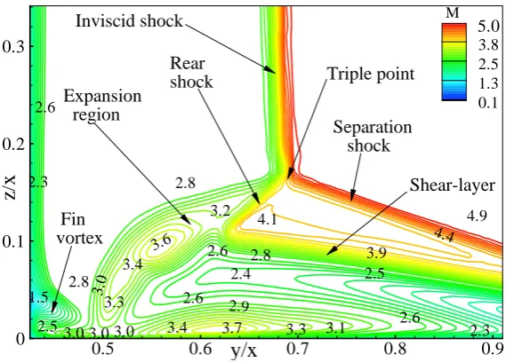
2.5 1.3 0.1 M

Separation shock Triple point Expansion

region

Shear-layer

5.0

Fin vortex

Rear shock Inviscid shock

Figure 7.Enlarged region of computed Mach contours at x-section = 122 mm.

The computed stagnation pressure contours in Figure5indicate that an inviscid shock bifurcates 144

and forms a separation shock and a rear shock, and results in the formation of lambda structure in a 145

cross plane perpendicular to the freestream flow direction. The shear-layer is formed over the vortex 146

region, which emanates from the separation point. It interacts with the rear shock-wave and then 147

rolls up and turns back to form a tongue. An entropy layer is generated from the triple point of the 148

intersection of three shock waves and a set of compression and expansion waves are formed between 149

the shear layer and the slip line (see Figure7). A secondary flow separation region was observed in 150

the experiments [19], whereas in the present computation, it is not predicted. The computed pressure 151

contours in Figure6indicate that an expansion fan is generated when the rear shock-wave reflects 152

from the shear layer. The computed Mach contours in Figure7 shows that a type-IV shock-shock 153

interaction [24] is observed at the triple point. An alternate increase and decrease in Mach contours in 154

the region between shear layer and jet represents the weak compression and expansion waves. The 155

flow remains supersonic in the separated region. Small subsonic pockets are observed near the corner 156

region of fin wall and plate. The impingement of the supersonic jet (entropy layer) emanating from 157

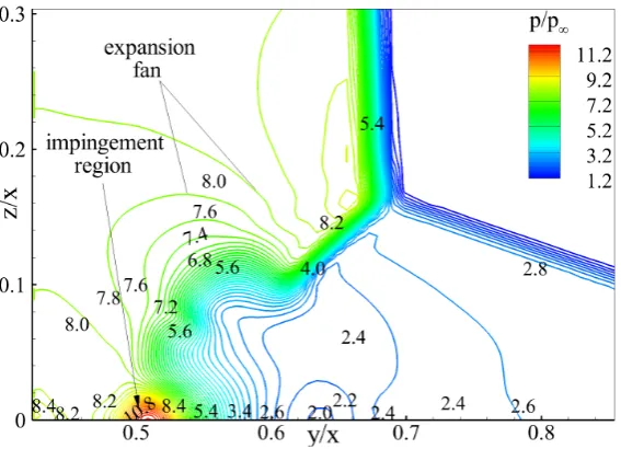
the triple pointof shock-shock interaction results in peak values of pressure as indicated in the region 158

marked in Figure6. A small fin-vortex is formed when the fluid coming from the inviscid region 159

interacts with fin wall and turns in the clockwise direction, as viewed from the downstream direction. 160

Similar, corner-vortex was observed in the vapor screen images of the experiments [4]. The schematic 161

5. Comparison of computed wall data with experiments 163

Figure 8.Computed pressure contours overlapped with wall pressure at x-section = 122 mm.

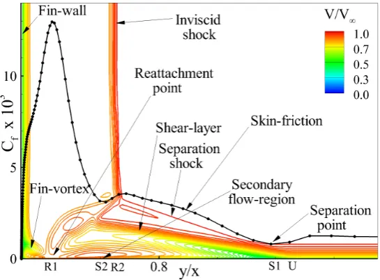
Figure 9.Computed speed contours overlapped with skin friction coefficient at x-section = 122 mm.

Figures8and 9 shows the computed pressure and speed contours, overlapped with the wall 164

pressure and skin friction on the flat plate at x-section = 122 mm. The distance along the y-axis is 165

normalized with the corresponding x-section distance measured from the fin tip. The surface data 166

is taken along the dashed lines as shown in Figure 1. The wall pressure remains constant in the 167

undisturbed boundary-layer before the interaction region. The separation shock affects the upstream 168

flow at the point of influence U and the wall pressure rises effectively across the separation shock 169

at primary separation point S1. It remains constant in the separated vortex flow and rises to peak 170

values at primary reattachment R1. The wall pressure then decreases away from the reattachment 171

region and rises near the fin-plate junction. The skin friction does not vary significantly in the 172

unperturbed boundary-layer before the region of influence U. The boundary-layer is compressed 173

friction. The skin friction reaches a peak value at the reattachment point R1 due to the high values of 175

the velocity gradient, hence shear stress. 176

Figure 10.Comparison of computed wall pressure at x-section = 152 mm with experiments [19] using

standard Spalart-Allmaras (SA) model [18] and modified Spalart-Allmaras model [16].

Figure 11.Comparison of computed skin friction at x-section = 122 mm with experiments [19] using

standard Spalart-Allmaras (SA) model [18] and modified Spalart-Allmaras model [16].

Figure10indicates that at x-section = 152 mm, experiments give an initial pressure rise location 177

at y/x = 1.22, where as the standard Spalart-Allmaras model predicts a delayed separation at y/x = 178

1.14. A similar trend is observed by the standard model at all other x-sections as shown in Table1. A 179

vortex region is calculated based on the distance between S1 and R1. The standard Spalart-Allmaras 180

model predicts a small vortex region of 74 mm as compared to the experimental value of 82 mm. The 181

skin friction coefficient predicted by the standard model in Figure11matches close to the experiments, 182

except in the secondary flow separation region. The model also under-predicts the peak values in the 183

reattachment region. 184

The shock-unsteadiness correction of [16] is applied to the complex region of three-dimensional 185

shock/boundary-layer interaction by evaluating the shock-unsteadiness parameter c′_b

1 in Eq.1. It 186

is a function of the upstream normal Mach number M1n and needs to be evaluated at each shock

187

wave so as to implement the shock-unsteadiness correction. The three-dimensional shock structure 188

in the single fin configuration is quite complex. It is not easy to find the orientation of the different 189

shock waves and the inclination of the upstream flow at each shock. Therefore, it is a difficult task 190

to calculate the mean value of M1n. An alternate approach is to use different values of c′_b1 in the

191

current single fin case to improve the flow predictions. A similar approach by Gaitonde et al. [27] was 192

used for simulating three-dimensional double-fin shock/boundary-layer interaction. The turbulence 193

model. A smaller value of model constant resulted in lower turbulent kinetic energy. Hence, the 195

computed solution resulted in a larger separated region and matched well with the experimental 196

flowfield and wall pressure. 197

3500

500 4500

6000 10500

2000

2500 2500

500

4000 1000

14500 8500

7000

y/x

z/

x

0.6 0.8 1 1.2

0.1

0.2 14000₉₅₀₀

5000 500

µ

/

µ

Figure 12. Computed normalized eddy-viscosity contours at x-section = 122 mm using standard

Spalart-Allmaras model [18].

3000

500 4500

6000 10500

2000

2500 2000

500

3000 1000

14500 8500 6500

y/x

z/

x

0.6 0.8 1 1.2

0.1

0.2 14000₉₅₀₀

5000 500

µ

/

µ

Figure 13. Computed normalized eddy-viscosity contours at x-section = 122 mm using

shock-unsteadiness modified Spalart-Allmaras model [16].

Table 1. Comparision of primary separation point S1 and reattachment point R1 using standard

Spalart-Allmaras (SA) and shock-unsteadiness modified SA model with the experiments [19] at different x-sections on the flat plate.

S1 R1

x-section, experiment SA modified experiment SA modified

mm SA SA

82 1.3 1.24 1.3 - 0.5 0.5

92 1.27 1.22 1.27 - 0.51 0.51

122 1.23 1.16 1.21 - 0.51 0.51

152 1.22 1.14 1.2 0.52 0.52 0.52

162 - 1.13 1.18 - 0.51 0.51

182 - 1.12 1.15 0.52 0.52 0.52

In the present case, a shock-unsteadiness parameter of c′_b

1 = -0.2 is chosen to yield a larger 198

separation and is found to match the experimental initial pressure rise location closely as indicated in 199

Figure10. The shock-unsteadiness correction reduces the turbulent eddy viscosity in the region of the 200

separation shock. This causes an increase in the length of the separation shock and hence brings the 201

separation point predictions close to the experiments. The same trend is observed in the axisymmetric 202

Figures12and 13indicate that the modification predicts lower values ofµT/µ∞in the region of

204

y/x≃1.2, as compared to the standard Spalart-Allmaras model. Hence, the modified model improves 205

the initial pressure rise location S1 (see Figure10). Also, the pressure distribution is well predicted 206

in the reattachment region and the corner region of the plate fin junction by the modified model as 207

compared to the standard model. 208

Figure11depicts that the modified model over predicts the skin friction between y/x = 0.65 and 209

0.72. Whereas, it under predicts the skin friction by 42% at the reattachment region R1. Panaras [15] 210

attributed this under prediction of skin friction due to the poor performance of turbulence models. 211

The models indicated lower values of turbulence inside the separation vortices, making the flow 212

almost laminar in this region. More advanced two-equation turbulence models [16? ? ] can be 213

applied to capture the velocity gradients, hence predict the peak skin friction at the reattachment 214

region accurately. Currently, this is beyond the scope of work. The modified Spalart-Allmaras model 215

predicts vortex region length between S1 and R1 to be 79 mm which is close to the experiment. The 216

computed locations of primary separation point S1 and reattachment point R1 are compared with the 217

experimental data at different x-sections in Table1. Overall, the modified Spalart-Allmaras model 218

matches to the experimental data at all locations. 219

6. Conclusion 220

Reynolds-averaged Navier-Stokes based computations were carried out to investigate the 221

three-dimensional shock/boundary-layer interaction in a single fin configuration at Mach 5 with 222

a large deflection angle of 23◦. The shock-unsteadiness modified Spalart-Allmaras model and its 223

standard version are used in the computations. The inviscid shock generated by the fin interacts 224

with the boundary layer on the adjacent flat plate and results in a formation of a complex region. 225

The viscous effects cause the bifurcation of inviscid shock and result in the formation of a lambda 226

shock structure, one edge being the separation shock and the other being the rear shock. Type-IV 227

shock-shock interaction results from the interaction of these shock waves. The lambda shock encloses 228

a cross flow conical vortex. A shear-layer emanates from the separation point and interacts with the 229

rear shock-wave and then rolls up and turns back to form a tongue. An entropy layer is generated at 230

the triple point and a set of compression and expansion waves are embedded in it and the shear layer. 231

These flow features influence the wall pressure and skin friction and a correlation between them is 232

explained. The standard Spalart-Allmaras model predicts initial pressure location downstream of 233

experiments. The shock-unsteadiness correction leads to an improvement in prediction of the initial 234

pressure rise location. This leads to an accurate prediction of vortex size, hence the shock structure. 235

The skin friction is under predicted at reattachment region in comparison to experiments by both 236

the modified model and its standard version. This behavior is attributed to the poor performance of 237

these models due to the prediction of laminar flow in this region. Further improvements to the present 238

computations are envisaged by simulating the more advanced two-equation turbulence models. 239

7. Acknowledgment 240

The author would like to thank Prof. Krishnendu Sinha from Department of Aerospace 241

Engineering, Indian Institute of Technology Bombay, for his valuable guidance, help and selflessness 242

time investment to accomplish this work. 243

References 244

1. Bose, D., Brown, J. L., Prabhu, D. K., Gnoffo, P., Johnston, C. O., and Hollis, B. Uncertainty assessment 245

of hypersonic aerothermodynamics prediction capability. Journal of Spacecraft and Rockets200350(1) 12-18, 246

DOI. 247

2. Marvin, J. G., Brown, J. L., and Gnoffo, P. A. Experimental database with baseline CFD solutions: 2-d and 248

3. Yang Z. Large-Eddy simulation: past, present and the future.Chinese Journal of Aeronautics201528(1) 11-24, 250

DOI. 251

4. Kubota, H. and Stollery, J. An experimental study of the interaction between a glancing shock wave and a 252

turbulent boundary layer.Journal of Fluid Mechanics1982116431-58, DOI. 253

5. Alvi, F. S. and Settles, G. Physical model of the swept shock wave/boundary layer interaction flowfield. 254

AIAA Journal199230(9) 2252-2258, DOI. 255

6. Edwards, J. R. and Chandra, S. Comparison of eddy viscosity-transport turbulence models for 256

three-dimensional shock-separated flowfields.AIAA Journal199634(4) 756-763, DOI. 257

7. Panaras, A. G. The effect of the structure of swept-shock-wave/turbulent boundary-layer interactions on 258

turbulence modeling.Journal of Fluid Mechanics1997338203-230, DOI. 259

8. Thivet, F. Lessons learned from RANS simulations of shock wave/boundary layer interactions. AIAA 260

Paper 2002-0583, Jan. 2002. 261

9. Panaras, A. G. Calculation of flows characterized by extensive crossflow separation. AIAA Journal2004 262

42(12) 2474-2475, DOI. 263

10. Delery, J., Marvin, J. G. and Reshotko, E. Shock-wave boundary layer interactions. AGARDograph No. 280, 264

ISBN 92-835-159-6, 1996. 265

11. Panaras, A. G. Review of the physics of swept-shock/boundary layer interactions. Progress in Aerospace 266

Sciences199632173-244, DOI. 267

12. Knight, D. D., and Degrez, G. Shock wave turbulent boundary layer interactions in high mach number 268

flows–a critical survey of current numerical prediction capabilities. AGARD Advisory Report1998319(2) 269

pp. 1.1-1.35. 270

13. Knight, D., Yan, H., Panaras, A. G., and Zheltovodov, A. Advances in CFD prediction of shock wave 271

turbulent boundary layer interactions.Progress in Aerospace Sciences200339(2-3) 121-184, DOI. 272

14. Babinsky, H. and Harvey, J. K. InShock wave-boundary-layer interactions; Cambridge University Press, 2011. 273

15. Panaras, A. G. Turbulence modeling of flows with extensive crossflow separation. Aerospace20152(3) 274

461-481, DOI. 275

16. Sinha, K., Mahesh, K., and Candler, G. V. Modeling the effect of shock-unsteadiness in shock/turbulent 276

boundary-layer interactions.AIAA Journal200543(3) 586-594, DOI. 277

17. Pasha, A. A., and Sinha, K. Shock-unsteadiness model applied to hypersonic shock wave/turbulent 278

boundary-layer interactions.Journal of Propulsion and Power201228(1) 46-60, DOI. 279

18. Spalart, P. R., and Allmaras, S. R. A one-equation turbulence model for aerodynamic flows. AIAA Paper 280

1992-0439, 1992. 281

19. Schulein, E. Optical skin friction measurements in short-duration facilities. AIAA Journal 2006 44(8) 282

1732-1742, DOI. 283

20. Wilcox, D. C. InTurbulence modeling for CFD; La Canada, CA: DCW Industries, 2nded., 2000, pp. 491-492. 284

21. Sinha. K., Candler G.V., Convergence improvement of two-equation turbulence model calculations. AIAA 285

Paper,AIAA-98-2649, 1998. 286

22. Pasha, A. A. and Sinha, K. Shock-Unsteadiness model applied to oblique shock-wave/turbulent 287

boundary-layer interaction.International Journal of Computational Fluid Dynamics200822(8) 569-582, DOI. 288

23. siva:2009 Reddy, D. S. K. and Sinha, K. Hypersonic turbulent flow simulation of fire II re-entry vehicle 289

afterbody.Journal of Spacecraft and Rockets200946(4) 745-757, DOI. 290

24. Edney, B. E. Anomalous heat transfer and pressure distributions on blunt bodies at hypersonic speeds in 291

the presence of an impinging shock. The Aeronautical Research Institute of Sweden, Stockholm, FFA Rept. 292

115, Feb. 1968. 293

25. Catris, S. and Aupoix, B. Density corrections for turbulence models. Aerospace Science and Technology2000 294

4(1) 1-11, DOI. 295

26. Deck, S., Duveau, P., d’Espiney, P., and Guillen, P. Development and application of SpalartAllmaras 296

one-equation turbulence model to three-dimensional supersonic complex configurations.Aerospace Science 297

and Technology20026(3) 171-183, DOI. 298

27. Gaitonde, D. V. Progress in shock-wave/boundary-layer interactions. Progress in Aerospace Sciences2015 299

72180-99, DOI. 300

28. Quadros, R., Sinha, K., and Larsson, J. Turbulent energy flux generated by shock/homogeneous turbulence 301

29. Quadros, R., and Sinha, K. Modelling of turbulent energy flux in canonical shock-International Journal of 303