Semantic Document Clustering Using a
Similarity Graph
Lubomir Stanchev
Computer Science Department California Polytechnic State UniversitySan Luis Obispo, California, USA e-mail: [email protected]
Abstract—Documentclusteringaddressestheproblemof iden-tifyinggroups ofsimilardocumentswithouthumansupervision. Unlikemostexistingsolutionsthatperformdocumentclustering based on keywords matching, we propose an algorithm that considers the meaning of the terms in the documents. For example, a documentthat contains thewords “dog” and“cat” multipletimesmaybeplacedinthesamecategoryasadocument that contains the word“pet” even if the two documents share onlynoisewordsincommon.Oursemanticclusteringalgorithm is basedonasimilarity graph thatstores thedegreeofsemantic relationship betweenterms (extracted from WordNet),wherea term can be a word or a phrase. We experimentally validate ouralgorithmontheReuters-21578benchmark,whichcontains
11,362newswirestoriesthatare groupedin82categoriesusing human judgment.Weapply thek-means clustering algorithmto group thedocuments usingasimilaritymetric thatis basedon keywords matchingandone that usesthe similaritygraph. We show that the second approach produces higher precision and recall,whichmeansthatthisapproachmatchesclosertheresults of thehumanstudy.
I. INTRODUCTION
Consider a web portal for an online store. To simplify nav-igation, merchandise may be grouped into categories. When a new product is introduced, it will be beneficial if the system can automatically classify the product in the correct category. This classification can be performed based on the description of the product. For example, consider a product with the following text description: “white sneakers, size 10”. If the system contains the knowledge that the terms “sneakers” and “athletic shoes” are related, then it can classify the new product in the “athletic shoes” category. In this paper, we show how such semantic knowledge can be stored in a similarity graph
and how it can be used to cluster documents based on the meaning of terms in their text.
The problem of semantic document clustering is interesting because it can improve the quality of the clustering result as compared to keywords-matching algorithms. For example, the later algorithm will likely put documents that use different terminology to describe the same concept in separate cate-gories. Consider a scientific document that contains the term “ascorbic acid” multiple times and a scientific document that contains the term “vitamin C” multiple times. The documents are semantically similar because “ascorbic acid” and “vitamin C” refer to the same organic compound and therefore the clus-tering algorithm should take this fact into account. However,
this will only happen when the close relationship between the two terms is stored in the system and used during document clustering. The need for a semantic clustering system becomes even more apparent when the number of documents is small or when they are very short. In this case, it is likely that the documents will not share many words in common and a keywords-matching system will struggle to find evidence for grouping documents together.
The problem of semantic document clustering is difficult because it involves some understanding of the meaning of words and phrases and how they interact. Although significant effort has been put forward in automated natural language processing [9], [10], [24], current approaches fall short of understanding the precise meaning of human text. In fact, whether computers will ever become as fluent as humans in understanding natural language text is an open problem. In this paper, we do not analyze natural language text and break it down into the parts of speech. Instead, we only consider the words and phrases in the documents and use the similarity graph, which is based on a probabilistic model, to compute the distance between pairs of documents. Note that, as described in the next paragraph, most clustering algorithms rely on a distance metric to cluster the documents.
A traditional keywords-matching algorithm for document clustering falls short because it only considers the words and their frequencies in each document. For example, the popular
k-means clustering algorithm [23] starts with k document seeds. It then finds the documents that are closest to each seed using a distance metric. Next, the centroid (i.e., mean) of each cluster is found and then new clusters are created using the centroids as the seeds. The process repeats and it is guaranteed to converge. The algorithm is based on a vector representation of the documents (based on words frequencies) and a distance metric (e.g., the cosine similarity between two document vectors). Unfortunately, this approach will incorrectly compute the similarity distance between two documents that describe the same concept using different words. It will only consider the common words and their frequencies and it will ignore the meaning of the words. Conversely, our approach adds all the documents to the similarity graph. The distance between a pair of documents is measured by evaluating the paths between them, where a path in the graph can go through several terms that are semantically similar. In this way, we consider not only Stanchev, 2016. Published in 2016 IEEE Tenth International Conference on Semantic Computing (ICSC), 1-8.
words, but also phrases (a.k.a. terms) that consist of several words. We also consider the meaning of these phrases.
Our approach for semantic document clustering is based on a similarity graph that was described in [38]. The graph uses mainly information from WordNet to find the degree of semantic similarity between 150,000 of the most common terms in the English language. The edges in the graph are asymmetric, where an edge between two nodes represents the probability that someone is interested in the concept that is described by the destination node given that they are interested in the concept that is described by the source node. Our approach adds the documents as nodes in the graph. They are connected to the graph based on the terms in them. For example, a document that contains the word “cat” will be connected to the word “cat”, which in tern is connected to the word “feline”, which in tern can be connected to a document that contains the word “feline”. In this way, our algorithm can compute the semantic distance between two documents by evaluating the degree of similarity between pairs of terms that appear in the documents.
When computing the similarity distance between two doc-uments, we aggregate the evidence from all the paths be-tween the first and the second document. Every path provides additional evidence about the similarity between the two documents. Note that the weight of a path decreases as the length of the path increases because longer paths provide weaker evidence. Since the paths in the graph are directed, we also examine the paths from the second to the first document and average the aggregated results.
We experimentally validate our document clustering algo-rithm on the Reuters-21578 benchmark. Out f the 21,578 newswire stories, 11,362 are categories in one of several categories using human judgment. Since our algorithm is based on hard clustering, that is every document can belong to at most one category, we consider only the first human classi-fication for each of the documents. We compare the results from the human judgment to applying the k-means clustering algorithm with two different distance metrics. The first is based on the popular cosine similarity metric that compares two documents as the cosine of the angle between the document vectors. The second metric is based on the distance between the documents in the similarity graph. We use the F-measure, which is popular in the research community [29], to evaluate how the results from the clustering algorithms compare to those of human judgment. The metric takes into account the number of documents that were correctly and wrongly classified to the same class and the number of documents that were wrongly assigned to different classes. When we apply the second distance metric, we get a higher value for the F-measure. This means that by using the similarity graph we can produce results that more closely match human judgment. The reason is that the similarity graph metric considers the meaning of the words and terms in the documents, while the cosine similarity metric only considers the words and their frequencies.
In what follows, in Section II we present a brief overview
of related research. The next section describes the similarity graph and presents example scenarios for creating the graph. While Section IV explains how to measure the semantic similarity between terms, Section V describes how to measure the semantic similarity between documents. Our main contri-butions are in the next two sections. Section VI describes two algorithms for clustering documents: using keywords matching and using the similarity graph. Section VII validates our semantic clustering algorithm by showing how it can produce data of better quality than the algorithm that is based on simple keywords matching. Lastly, Section VIII summarizes the paper and outlines areas for future research.
II. RELATED RESEARCH
A plethora of research has been published on using su-pervised learning models with training sets for document classification [5], [40]. Our approach differs because it is unsupervised, it does not use a training set, and it can cluster documents in any number of classes rather than just classify the documents in preexisting topics.
One alternative to supervised learning is using a knowledge-base that contains information about the relationship between the words and phrases that can be found in the documents to be clustered. For example, in 1986, W. B. Croft proposed the use of a thesaurus that contains semantic information, such as what words are synonyms [7]. Sequentially, there have been multiple papers on the use of a thesaurus to represent the semantic relationship between words and phrases [13], [14], [15], [17], [19], [27], [32], [41]. This approach, although very progressive for the times, differs from our approach because we consider indirect relationships between words (i.e., relationships along paths of several words). We also do not apply document expansion (e.g., adding the synonyms of the words in a document to the document) when comparing two documents. Instead, we use the similarity graph to compute the distance between two documents. Some limited user interac-tion is possible when classifying documents – see for example the research on folksonomies [11]. Our system currently does not allow for user interaction when creating the document clusters.
In later years, the research of Croft was extended by creating a graph in the form of a semantic network [4], [30], [33] and graphs that contain the semantic relationships between words [2], [1], [6]. Later on, Simone Ponzetto and Michael Strube showed how to create a graph that only represents inheritance of words in WordNet [21], [34], while Glen Jeh and Jennifer Widom showed how to approximate the similarity between phrases based on information about the structure of the graph in which they appear [18]. All these approaches differ from our approach because they do not consider the strength of the relationship between the nodes in the graph. In other words, there are no weights that are assigned to the edges in the graph. Natural language techniques can be used to analyze the text in a document [16], [26], [36]. For example, a natural language analyzer may determine that a document talks about animals and words or concepts that can represent an animal
can be identified in other documents. As a result, documents that are identified to refer to the same or similar concepts can be classified together. One problem with this approach is that this is computationally expensive. A second problem is that it is not a probabilistic model and therefore it is difficult to be applied towards generating a document similarity metric.
Ontologies can be used for document classification [31]. Our approach is different because we do not consider pres-elected categories. Using ontologies also requires manual or automatic annotation of each document with a description in a formal language [20], [28], [12]. This may be problematic because manual annotation is time consuming and automatic annotation is not very reliable.
Since the early 1990s, research on LSA (stands for latent semantic analysis [8]) has been carried out. The approach has the advantage of not relying on external information. Instead, it considers the closeness of words in text documents as proof of their semantic similarity. For example, LSA can be used to detect words that are synonyms [22]. This differs from our approach because we do not consider the closeness of words in a document. The only time we consider the position of words is when we examine the order of the words in the definition of a WordNet sense when we build the similarity graph, where we assume that the first words are more important. Although the LSA approach has its applications, we believe that our sources of knowledge, such as WordNet, provide data of higher quality.
III. CREATING THE SIMILARITY GRAPH
In this section, we review how the similarity graph can be created using information from WordNet [25], where we encourage the reader to refer to [38] for a more detailed description. WordNet gives us information about the words in the English language. The similarity graph is initially constructed using WordNet 3.0, which contains about 150,000 different terms. Both words and phrases can be found in WordNet. For example, “sports utility vehicle” is a term from WordNet. We will sometimes refer to these words and phrases as terms, while WordNet uses the terminology word form. Note that the meaning of a term is not precise. For example, the word “spring” can mean the season after winter, a metal elastic device, or natural flow of ground water, among others. This is the reason why WordNet uses the concept of a sense. For example, earlier in this paragraph we cited three different senses of the word “spring”. Every word form has one or more senses and every sense is represented by one or more word forms. A human can usually determine which of the many senses a word form represents by the context in which the word form is used. WordNet contains about 116,000 senses for the 150,000word forms.
The initial goal of the similarity graph is to model the rela-tionship between the terms in WordNet using a probabilistic model. The weight of an edge between two nodes represents the probability that a user is interested in documents that contain the label of the destination node given that they are interested in the label of the source node. For every term that is not a noise word, a node that has the term as a label is
created. Similarly, for every sense we create a node with a label that is the description of the sense. All node labels are converted to lower case and we do not create multiple nodes with the same label.
As expected, we join every word form node with the sense nodes for the word form using edges. We also join a sense node with the nodes for the non-noise words in the description of the sense using edges, where higher weights are given to the first words. The reason is that we believe that there is a greater chance that a user will be interested in one of the first words in the definition of a sense given that they are interested in the sense. For example, the most popular sense of the word “chair” is “a seat for one person”. There is obviously a strong relationship between the words “chair” and “seat”, which is extracted by the algorithm. Similarly, WordNet contains example use for each sense and the similarity graph contains an edge between each sense and each non-noise word in its example use. As expected, the weights of these edges are smaller than the weights for the definition edges because the definition of a sense provides stronger evidence than the example use of a sense about the degree of semantic relevance. WordNet also contains a plethora of information about the relationship between senses. The senses in WordNet are divided into four categories: nouns, verbs, adjectives, and adverbs. For example, WordNet stores information about the
hyponym and meronym relationship for nouns. The former corresponds to the “kind-of” connection (e.g., “dog” is a hyponym of “canine”). The later corresponds to the “part-of” relationship (e.g., “window” is a meronym of “building”). Similar relationships are also defined for verbs, adjectives, and adverbs. For each such relationship, the similarity graph contains an edge between the sense nodes, where the weight of the edge depends on the likelihood that a user will be interested in the destination sense given that they are concerned about the source sense. The relationship between two terms is determined as a function of the relationship between their senses.
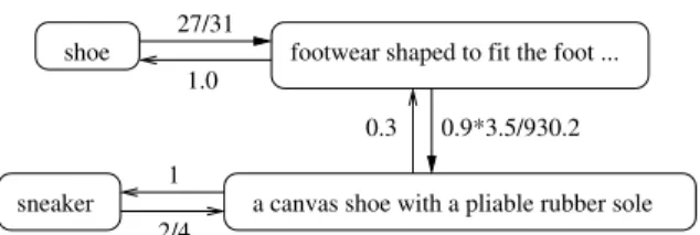
Instead of presenting a detailed description of how the weights of the edges are extracted from WordNet (this infor-mation can be found in [38]), we show some previously un-published examples. First, consider Fig. 1. The edge between the word “shoe” and its main sense has weight 27/31 because WordNet defines five senses of the word “shoe”. The main sense is shown in the figure and WordNet gives it a frequency value of 27, where all the other senses of the word have a frequency of one. In other words, the sum of the frequencies of all senses, according to WordNet, is 31 and therefore there is a 27/31 chance that someone who is interested in the word “shoe” will also want to know about the most popular sense of the word. The backward edge has weight of one because there is a 100%probability that someone who is interested in a sense is also concerned about the words that describes it.
The edge between the two senses represents the hypernym
relationship (the reverse of the hyponym relationship). In other words, sneaker is a type of shoe. Our algorithm tries to find the “size” of the two senses. For the word “shoe”, we consider all
the hypernyms and add their sizes. Suppose the result is 930.2. This information is computed with the help of the British National Corpus (BNC) [3], which tells us the frequency of use of the words in the English language. For example, the word “sneaker” has four senses, where the main sense that we are interested in has a frequency of two and the other two senses have frequency of one. Suppose that BNC tells us that the frequency of the word “sneaker” is seven. Then the size the sense that is in the figure is 7∗(2/4) = 3.5. Note that, for simplicity, in our example we did not consider the other terms that represent the sense for the word “sneaker” (such as “gym shoe”) and doing so increases the size of the sense. By dividing the size of the sense for the word “sneaker” by the size of the sense for word “shoe”, we get an approximate idea of how likely it is that someone who is interested in shoes is also concerned about sneakers. We believe that there is a 90% chance that someone who is interested in a sense will also want to get information about one of it hypernyms. Note that throughout the paper we use several such constants and [38] shows that these numbers can produce graph data of good quality. As Fig. 1 suggests, our formula for the hypernym relationship is 0.9 times the size of the destination sense and divided by the size of the source sense. Note that the size of the later is calculated as the sum of the sizes of all its hypernyms. The backward edge between the two nodes has weight of 0.3, which is the weight that we assign to all hyponym (i.e., kind-of) relationships in the graph.
Lastly, the weight of the edge between the main sense of the word “sneaker” and the word “sneaker” is one because the sense represents the word. In other words, there is a 100% probability that someone who is interested in a sense will also want to know about one of the terms that represents it. The backward edge has weight 2/4 and corresponds to the fact that there are three senses of the word sneaker: “a canvas shoe with a pliable rubber sole”, ”someone acting as an informer or decoy for the police”, and “marked by quiet and caution and secrecy” and the main sense has frequency of two, while the other two senses have a frequency of one.
In order to compute the relevance score between the words “shoe” and “sneaker”, we need to multiply the weights of all the edges along the forward path. If there are multiple paths between the words, then we compute the product of the weights of the edges along each path and then we aggregate the evidence. Note that there is also a reverse paths from the word “sneaker” to the word “shoe”. Our algorithm considers paths in both directions and then it averages the results (see Section IV for more details). Based only on Fig. 1, the weight of the
0.9·3.5
forward path will be 27 31 · 930.2 ·1and the weight of backward path will be 2 4 ·0.3·1. The average of the two numbers will give us an idea about the strength of the relationship between the two concepts.
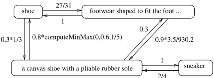
There is a second path in the graph between the words “shoe” and “sneaker”. As shown in Fig. 2, the word “shoe” ap-pears in the definition of the main sense of the word “sneaker”. Assume that the word “shoe” appears in the definition of exactly three senses. We will then draw a forward edge with
0.3
shoe footwear shaped to fit the foot ...
a canvas shoe with a pliable rubber sole sneaker 0.9*3.5/930.2 1.0 27/31 1 2/4
Fig. 1. Example relationship between the words “shoe” and “sneaker” along the hypernym relationship.
1
weight 0.3·3 . The constant 0.3represents that we approximate that there is a 30% probability that a user that is interested in a term will also want to know about one of the senses that contains the term in its definition. In [39], we have experimentally shown that this number produces a graph with good quality data. The ratio 1 3 is based on the fact that there are three different sense definitions that contain the word “shoe”.
0.8*computeMinMax(0,0.6,1/5) shoe
a canvas shoe with a pliable rubber sole sneaker
0.3*1/3 1 2/4
Fig. 2. Example relationship between the words “shoe” and “sneaker” along the words-in-sense-definition relationship.
The backward edge between the two words uses the
computeMinMax function. We use the function every
time we consider the frequency of terms inside text. The
computeMinMax function returns a number that is almost always between the first two arguments, where the magnitude of the number is determined by the third argument. The last parameter is the number of times a word appears in the text divided by the total number of words. In our example, we only consider the non-noise words in the definition of the sense and therefore the value of the third parameter is 1/5 because “shoe” is one of the five non-noise words in the definition of the main sense for the word “sneaker”. The second parameter (i.e., 0.6) is a constant that represents how likely it is for someone to be interested in one of the words in the definition of a sense given that they are interested in the sense. The computeMinMax function smoothens the value of the third parameter. For example, a word that appears as one of 20 words in the definition of a sense is not 10 times less important than a word that appears as one of two words in the definition. The function makes the difference between the two cases less extreme. Using this function, the weight of the edge in the second case will be only roughly four times smaller than the weight of the edge in the first case. This is a common approach when processing text. The importance of a word in a text decreases as the size of the text increases, but the importance of the word decreases slower than the rate of growth of the text. Formally, the function computeMinMax is defined as follows.
w1 →sw2 +w2 →sw1 1
|w1, w2|lin=min(α, )∗ (3)
2 α
computeMinMax(minValue,maxValue,ratio) = −1
minValue+ (maxValue−minValue)∗log2(ratio)
−1
|w1, w2|log=norm( ) (4) log2(min(α,w1→sw2+w2→sw1))
2 Note that when raio = 0.5, then the function returns
max-Value. An unusual case is when the value of the variable ratio
is bigger than 0.5. For example, if ratio = 1, then we have division by zero and the value for the function is undefined. We handle this case separately and assign value to the function equal to 1.2∗maxValue. This is an extraordinary case when there is a single non-noise word in the text description and we need to assign higher weight to the edge.
We multiply the backward edge by 0.8 because “shoe” is the second non-noise word in the definition of the sense. Our algorithm multiplies the first non-noise word by one and the coefficient is decreased by 0.2 for every sequential word until it reaches 0.2. This strategy is based on our belief that the first words in the definition of a sense are more important, where [39] experimentally validates this belief.
2/4 shoe
a canvas shoe with a pliable rubber sole sneaker 0.3*1/3 0.8*computeMinMax(0,0.6,1/5)
footwear shaped to fit the foot ... 27/31
1
0.3
0.9*3.5/930.2
1
Fig. 3. Example relationships between the words “shoe” and “sneaker”.
Fig. 3 shows the result of combining the two graph. In the figure, there are two forward paths from the word “shoe” to the word “sneaker”. If we add the evidence from the two paths, then we get the number 27 ·0.9·3.5·1 + 0.3∗1·1
31 930.2 3 . Similarly,
from the backward paths we will collect additional evidence about the similarity of the two words: 24 ·0.3·1 + 24 ·0.8·
computeMinMax(0,0.6,15 ). As we add evidence from several paths, the weight for a path can become bigger than one and therefore cease to represent a probability. In the next section, we address this issue by capping the similarity score between two nodes in the graph.
IV. MEASURING THE SEMANTIC SIMILARITY BETWEEN ERMS
T
The similarity graph is used to represent the conditional probability that a user is interested in the term that is described by the label of a node given that they are also interested in the label of an adjacent node in the graph. We compute the directional similarity between two nodes using the following formula.
X
A→sC= PPt(C|A) (1)
Pt is a cycleless path from node A to node C
Y
PPt(C|A) = P(n2|n1) (2) (n1,n2) is an edge in the path Pt
The function P(n2|n1) refers to the weight of the edge from the node n1 to the node n2. Informally, we compute the directional similarity between two nodes as the sum of the weights of all the paths between the two nodes, where we eliminate cycles from the paths. Each path provides evidence about the similarity between the terms that are represented by the two nodes. We compute the weight of a path between two nodes as the product of the weights of the edges along the path, which follows the Markov chain model. Since the weight of an edge along the path is almost always smaller than one (i.e., equal to one only in rear circumstances), the value of the conditional probability will decrease as the length of the path increases. This is a desirable behavior because a longer path provides less evidence about the similarity of the two end nodes. For alternative ways of computing the directional similarity between two nodes, see [39].
Next, we present two functions for measuring the semantic similarity between two nodes. The linear function for com-puting the semantic similarity between two nodes is shown in Equation 3.
The minimum function is used in order to cap the value of the similarity function at one. The coefficient αamplifies the available evidence (α≤1). Note that when αis equal to one, then the function simply takes the average of the two numbers and caps the result at 1.
The second similarity function is inverse logarithmic, that is, it amplifies the smaller values. It is shown in Equation 4. The norm function simply multiplies the result by a constant (i.e., −log2(α)) in order to move the result value in the range [0,1].
The paper [39] suggests that the two similarity metrics produce best results when αis around 0.1 and this is the value that we will use in the experimental section.
V. MEASURING THE SEMANTIC SIMILARITY BETWEEN
DOCUMENTS
In the previous section, we described how to measure the semantic similarity between two nodes of the graph. In this section, we describe how to measure the semantic similarity between any two text documents. The idea is to create a node for each document and then connect the nodes to the graph. The semantic similarity between two documents will then be measured by computing the distance between the two nodes using the linear or logarithmic algorithm from the previous section.
In order to demonstrate our approach, consider a fictitious document that contains a total of 10 non-noise words in its title and a total of 100 non-noise words in its body. Among these non-noise words, suppose that the word “sneaker” appears
~ ~ d1 ·d2
|d1, d2|cosine =
~ ~
|d1| ∗ |d2| once in the title and the word “shirt” is present four times
in the body. We will represent this information by drawing the graph that is shown in Fig. 4. The weight of the edge between the document and the word “sneaker” is equal to
computeMinMax(0,0.6,1/10)=0.18. Similarly, the weight of the edge between the document and the word “shirt” is
4
equal to computeMinMax(0,0.3,100 ) = 0.13. This is the same formula that is used to compute the weight of an edge between a sense and the words in its definition. The number 0.6is used because we believe that there is a high probability that someone who is interested in a document will also want information about one of the terms that appears in its title. The number 0.3 represents our belief that there is a 30% chance that someone who is interested in a document is also concerned about one of the terms that appear in its body. Here, we assume that the terms in the title of a document are twice as important as the terms in the body.
Next, consider the backward edge between the word “sneaker” and the document. Suppose that the word appears a total of 10 times in all documents. Then the weight of the edge between the word “sneaker” and the document will be
1
equal to 0.3·10 = 0.03. This is the same formula that is used for computing the weights of the backward edges between a word form from WordNet and the definition of the sense in which it appears. We believe that the backward edges are less important and therefore we divide the coefficients by two for backward edges (the coefficient for the forward edge is 0.6 as shown in the previous paragraph). Similarly, if the word “shirt” appears a total of 20 times in all documents, then we
4
will draw a backward edge with weight 0.15·20 = 0.03(the coefficient for the forward edge is 0.3 and the coefficient for the backward edge is half of that, that is, 0.15).
0.03 and 100 non−noise words in its body. The word "sneaker" appears once in the title and the word ‘‘shirt" appears four times in the body.
sneaker 0.13
shirt 0.18 0.03
Document with 10 non−noise words in its title
Fig. 4. Example of adding a document to the graph.
Although we consider the words in the title more important than the words in the body, we do not pay special attention to the order of the words. The reason is that there is no empirical evidence that the first words in the title or body of a document or more important.
The word “sneaker” has two different senses. Our algorithm does not try to identify which of these senses the document refers to. Instead, there will be paths in the graph to both senses. We take this approach because it can be possible that different occurrences of the word in the document refer to distinct senses. The strength of the relationship to a particular sense will be computed based on additional evidence. For example, if the document also contains the word “shoe”, then
there will be stronger connection between the document and the main sense of the word “sneaker”.
Second, note that the distance between two documents is not calculated in isolation. In particular, the other documents in the corpus are also taken into account when calculating the backward edges. In other words, we calculate how similar two documents are relative to the rest of the documents in the corpus. Once the similarity graph is extended with the documents, the distance between two documents can be calculated using the linear or logarithmic metrics that were described in the previous section.
VI. CLUSTERING THE DOCUMENTS
In this section we describe how a set of documents can be clustered using the k-means clustering algorithm. The algorithm relies on a way for computing the distance between two documents. We present two variations: using keywords matching and using the similarity graph. In the next section we show how the results of the two algorithms compare to human judgment.
A common approach for computing the similarity distance between two documents is to represent them as vectors and then compute the cosine of the angle between the two vectors as the normalized dot product of the vectors. For example, suppose that “dog”, “cat” and “shirt” are the only words that are used. Then for every document we can denote the number of times each word occurs. For example, a document that contains the word “dog” twice, the word “cat” three times and does not contain the word “shirt” can be represented as the document vector [2,3,0]. Alternatively, a document that contains the word “cat” twice and the word “shirt” four times can be represented as [0,2,4]. The dot product of the two vectors is [2,3,0]· [0,2,4] = 6. Next, we need to divide the result by the product of the sizes of the two documents. Therefore, the angle between the documents in radians will
6
be √ √ ≈ 0.37. Unfortunately, this approach
(22+32)∗ 22+42
does not take into account that the words “cat” and “dog” are semantically similar and will calculate the similarity distance between a document about cats and one about dogs as zero if the two documents do not share words in common. In general, the cosine similarity between two documents is computed using the formula in Equation 5. Alternatively, we can use the linear or logarithmic metric from the previous section to compute the semantic distance between two documents.
(5) The k-means clustering algorithm starts with a constant k. This is the number of clusters that will be produced. Initially, a centroid (i.e., a document) is randomly chosen for every cluster. Next, each document is assigned to the group that contains the closest centroid. After that, the centroid (i.e., mean) is found for each cluster and then the documents are clustered again around each centroid. The algorithm converges and continues until applying the last step does not change the
T P P =T P+F P T P R=T P +F N (β2+1)·P·R Fβ= β2·P +R clustering. If the documents are represented as vectors as we
showed earlier in this section, then computing the mean of a set of documents amounts to adding the document vectors and dividing by the number of documents. For example, the mean of our two document vectors from the beginning of this section
[2,5,4]
is mean([2,3,0],[0,2,4]) = 2 = [1,2.5,2]. Note that the mean function is independent of the document similarity metric that is used.
VII. EXPERIMENTAL RESULTS
All our code was implemented in Java. We first created the similarity graph using WordNet and it took about 10 minutes to create the graph on a standard laptop with Intel i5 CPU. We used the Java API for WordNet Searching (JAWS) to connect to WordNet. The interface was developed by Brett Spell [35]. We stored the graph as several Java hash tables, where the size of the file is 89MB.
We next read all the documents from the Reuters-21578 benchmark. The benchmark contains 21,578 documents that are stored in 22 text files. Our program read the files and we extracted information about the 11,362 documents that were classified in one of 82 categories using human judgment. For every document, we stored its title, its text, the category it belongs to, and a document vector. The later contains the non-noise words in the documents and their frequency. Since the words in the title are more important, we counted these words twice. We stored the information in Java hash tables, where the size of the file is 27MB. It took about two minutes to parse the text files.
We next added the documents to the similarity graph. We followed the algorithm from Section V and gave higher weights to the terms in the titles of the documents. The size of the graph increased to 129MB. For document nodes, we stored the title of the document in the label of the node. We also stored a hash table that keeps the mapping between the document nodes in the graph and the documents in the document file that was described in the previous paragraph. It took about five minutes to add the documents to the graph.
We next clustered the documents using the k-means clus-tering algorithm. We chose the value k = 82 because this is the number of categories as determined by the human judgment. The first 82 documents were put in 82 distinct clusters. At this point, the lonely document in each category was designed as the centroid. We next processed the rest of the documents. Every document was compared to the 82 centroids and assigned to the cluster with the closest centroid. Next, a new centroid was chosen for each cluster. This was done by adding the document vectors in each cluster and dividing the result by the number of vectors (i.e., finding the mean in each cluster). Next, the documents were reclustered around the new centroids and the process was repeated until it converged (i.e., applying the algorithm did not change the clusters).
The k-means clustering algorithm is based on two document functions: finding the distance between two documents and computing the average of several documents. The later func-tion is implemented by simply adding the document vectors
TABLE I
RESULTS OF APPLYING THE K-MEANS ALGORITHM cosine linear logarithmic # of rounds 30 45 45 precision 0.57 0.66 0.66 recall 0.05 0.07 0.07 F-measure 0.09 0.13 0.13
and dividing the result by the number of vectors. However, we have three choices for the distance metric: the cosine, linear, and logarithmic. When we applied the cosine similarity metric, the k-means clustering program terminated in about three hours and it took 30 rounds until ed paths of length more than three edges or weight less than 0.01 when computing the distance between two documents using the similarity graph. The results of using the three different distance metrics are shown in Table I.
The table shows the F-measure when using the three different distance metrics. The measure gives a single number based on the precision and recall of the result of the clustering algorithm. Let TP be the number of true positives, that is, the number of documents that were classified in the same category by both the program and human judgment. Let FP be the number of false positives, that is, the number of documents that were classified in the same category by the program, but were classified in different categories by human judgment. Lastly, let FN be the number of false negatives, that is, the number of documents that were classified in the same category by human judgment but were classified in different categories by the program. The formula for computing the F-measure is shown below.
In the above formulas, Pis used to denote the precision and
R is used to denote the recall. We used the value β = 1 in the experimental results, which is a popular parameter for the F-measure metric. As the table suggests, using the similarity graph can lead to both higher precision and recall. Note that using the linear or logarithmic similarity metric did not make a difference. The reason is that the two metrics apply different monotonic functions on the average of the sum of the forward and backward paths. Applying these monotonic functions has no effect on the ordering of the distances between nodes and on the clustering result.
VIII. CONCLUSION AND FUTURE RESEARCH
In this paper we reviewed how information from WordNet can be used to build a similarity graph. The graph shows the strength of the relationship between words and phrases from the English language. We showed how to use the graph to cluster documents. We validated the algorithm experimentally
by comparing it to an algorithm that uses the cosine similarity metric. Using the similarity graph leads to increased precision and recall on the popular Reuters-21578 benchmark.
One area for future research is using an extended version of the similarity graph that contains information from Wikipedia [37] to perform document clustering. One challenge in this area is that the extended graph is relatively big (more than 10GB) and computing the distance between documents can be computationally expensive.
REFERENCES
[1] M. Agosti and F. Crestani. Automatic Authoring and Construction of Hypertext for Information Retrieval. ACM Multimedia Systems, 15(24), 1995.
[2] M. Agosti, F. Crestani, G. Gradenigo, and P. Mattiello. An Approach to Conceptual Modeling of IR Auxiliary Data. IEEE International Conference on Computer and Communications, 1990.
[3] L. Burnard. Reference Guide for the British National Corpus (XML Edition). http://www.natcorp.ox.ac.uk, 2007.
[4] P. Cohen and R. Kjeldsen. Information Retrieval by Constrained Spreading Activation on Sematic Networks. Information Processing and Management, pages 255–268, 1987.
[5] R. Collobert and J. Weston. A Unified Architecture for Natural Language Processing: Deep Neural Networks with Multitask Learning. Twenty Fifth International Conference on Machine Learning, 2008.
[6] F. Crestani. Application of Spreading Activation Techniques in Infor-mation Retrieval. Artificial Intelligence Review, 11(6):453–482, 1997. [7] Croft. User-specified Domain Knowledge for Document Retrieval.
Nineth Annual International ACM Conference on Research and Devel-opment in Information Retrieval, pages 201–206, 1986.
[8] S. Deerwester, S. T. Dumais, G. W. Furnas, T. K. Landauer, and R. Harshman. Indexing by Latent Semantic Analysis. Journal of the Society for Information Science, 41(6):391–407, 1990.
[9] C. Fox. Lexical Analysis and Stoplists. Information Retrieval: Data Structures and Algorithms, pages 102–130, 1992.
[10] W. Frakes. Stemming Algorithms. Information Retrieval: Data Struc-tures and Algorithms, pages 131–160, 1992.
[11] T. Gruber. Collective knowledge systems: Where the social web meets the semantic. Web Journal of Web Semantics, 2008.
[12] R. V. Guha, R. McCool, and E. Miller. Semantic Search. Twelfth International World Wide Web Conference (WWW 2003), pages 700– 709, 2003.
[13] A. M. Harbourt, E. Syed, W. T. Hole, and L. C. Kingsland. The Ranking Algorithm of the Coach Browser for the UMLS Metathesaurus. Seventeenth Annual Symposium on Computer Applications in Medical Care, pages 720–724, 1993.
[14] W. R. Hersh and R. A. Greenes. SAPHIRE An Information Retrieval System Featuring Concept Matching, Automatic Indexing, Probabilistic Retrieval, and Hierarchical Relationships. Computers and Biomedical Research, pages 410–425, 1990.
[15] W. R. Hersh, D. D. Hickam, and T. J. Leone. Words, Concepts, or Both: Optimal Indexing Units for Automated Information Retrieval. Sixteenth Annual Symposium on Computer Applications in Medical Care, pages 644–648, 1992.
[16] E. H. Hovy, L. Gerber, U. Hermjakob, M. Junk, and C. Y. Lin. Question Answering in Webclopedia. TREC-9 Conference, 2000.
[17] K. Jarvelin, J. Keklinen, and T. Niemi. ExpansionTool: Concept-based Query Expansion and Construction. Springer Netherlands, pages 231– 255, 2001.
[18] G. Jeh and J. Widom. SimRank: A Measure of Structural-context Similarity. Proceedings of the Eight ACM SIGKDD International Conference on Knowledge Discovery and Data Mining, pages 538–543, 2002.
[19] S. Jones. Thesaurus Data Model for an Intelligent Retrieval System. Journal of Information Science, 19(1):167–178, 1993.
[20] A. Kiryakov, B. Popov, I. Terziev, D. Manov, and D. Ognyanoff. Se-mantic Annotation, Indexing, and Retrieval. Journal of Web Semantics, 2(1):49–79, 2004.
[21] R. Knappe, H. Bulskov, and T. Andreasen. Similarity Graphs. Fourteenth International Symposium on Foundations of Intelligent Systems, 2003.
[22] T. K. Landauer, P. Foltz, and D. Laham. Introduction to Latent Semantic Analysis. Discourse Processes, pages 259–284, 1998.
[23] J. B. MacQueen. Some Methods for Classification and Analysis of Multivariate Observations. Proceedings of Fifth Berkeley Symposium on Mathematical Statistics and Probability, page 281?297, 1967. [24] M.F.Porter. An Algorithm for Suffix Stripping. Readings in Information
Retrieval, pages 313–316, 1997.
[25] G. A. Miller. WordNet: A Lexical Database for English. Communica-tions of the ACM, 38(11):39–41, 1995.
[26] D. Moldovan, S. Harabagiu, M. Pasca, R. Mihalcea, R. Goodrum, and R. Girju. LASSO: A Tool for Surfing the Answer Net. Text Retrieval Conference (TREC-8), 1999.
[27] C. Paice. A Thesaural Model of Information Retrieval. Information Processing and Management, 27(1):433–447, 1991.
[28] B. Popov, A. Kiryakov, D. D. Ognyanoff, D. Manov, and A. Kirilov. KIM A Semantic Platform for Information Extraction and Retrieval. Journal of Natural Language Engineering, 10(3):375–392, 2004. [29] D. Powers. ”evaluation: From precision, recall and f-measure to
roc, informedness, markedness and correlation”. Journal of Machine Learning Technologies, 2(1):37?63, 2011.
[30] L. Rau. Knowledge Organization and Access in a Conceptual Informa-tion System. Information Processing and Management, 23(4):269–283, 1987.
[31] S. S. Luke, L. Spector, and D. Rager. Ontology-Based Knowledge Discovery on the World Wide Web. Internet-Based Information Systems: Papers from the AAAI Workshop, pages 96–102, 1996.
[32] M. Sanderson. Word Sense Disambiguation and Information Retrieval. Seventeenth annual international ACM SIGIR conference on Research and development in information retrieval, 1994.
[33] P. Shoval. Expert consultation system for a retrieval database with semantic network of concepts. Fourth Annual International ACM SIGIR Conference on Information Storage and Retrieval: Theoretical Issues in Information Retrieval, pages 145–149, 1981.
[34] Simone Paolo Ponzetto and Michael Strube. Deriving a Large Scale Taxonomy from Wikipedia. 22nd International Conference on Artificial Intelligence, 2007.
[35] B. Spell. Java API for WordNet Searching (JAWS). http://lyle.smu.edu/ tspell/jaws/index.html, 2009.
[36] K. Srihari, W. Li, and X. Li. Information Extraction Supported Question Answering. In Advances in Open Domain Question Answering, 2004. [37] L. Stanchev. Creating a Phrase Similarity Graph from Wikipedia. Eight
IEEE International Conference on Semantic Computing, 2014. [38] L. Stanchev. Creating a Similarity Graph from WordNet. Fourth
International Conference on Web Intelligence, Mining and Semantics, 2014.
[39] L. Stanchev. Measuring the Strength of the Semantic Relationship Between Words. International Journal on Artificial Intelligence Tools, 2015.
[40] J. Turian, L. Ratinov, and Y. Bengio. Word representations: A simple and general method for semi-supervised learning. In Forty Eight Anual Meeting of the Association for Computational Linguistics, pages 384– 394, 2010.
[41] Y. Yang and C. G.Chute. Words or Concepts: The Features of Indexing Units and their Optimal use in Information Retrieval. Seventeenth Annual Symposium on Computer Applications in Medical Care, pages 685–68, 1993.