Pricing stock options under stochastic volatility and interest rates with efficient method of moments estimation

Pricing Stock Options

under Stochastic Volatility and Interest Rates

with Efficient Method of Moments Estimation

George J. Jiang∗and Pieter J. van der Sluis† 28th July 1999

∗ _{George J. Jiang, Department of Econometrics, University of Groningen, PO Box 800, 9700 AV}

Groningen, The Netherlands, phone +31 50 363 3711, fax, +31 50 363 3720, email: [email protected];

† _{Pieter J. van der Sluis, Department of Econometrics, Tilburg University, P.O. Box 90153, NL-5000}

LE Tilburg, The Netherlands, phone +31 13 466 2911, email: [email protected]. This paper was presented at the Econometric Institute in Rotterdam, Nuffield College at Oxford, CORE Louvain-la-Neuve and Tilburg University.

Abstract

While the stochastic volatility (SV) generalization has been shown to improve the explanatory power over the Black-Scholes model, empirical implications of SV models on option pricing have not yet been adequately tested. The purpose of this paper is to first estimate a multivariate SV model using the efficient method of moments (EMM) technique from observations of underlying state variables and then investigate the respective effect of stochastic interest rates, systematic volatility and idiosyncratic volatility on option prices. We compute option prices using reprojected underlying historical volatilities and implied stochastic volatility risk to gauge each model’s performance through direct comparison with observed market option prices. Our major empirical findings are summarized as follows. First, while theory predicts that the short-term interest rates are strongly related to the systematic volatility of the consumption process, our estimation results suggest that the short-term interest rate fails to be a good proxy of the systematic volatility factor; Second, while allowing for stochastic volatility can reduce the pricing errors and allowing for asymmetric volatility or “leverage effect” does help to explain the skewness of the volatility “smile”, allowing for stochastic interest rates has minimal impact on option prices in our case; Third, similar to Melino and Turnbull (1990), our empirical findings strongly suggest the existence of a non-zero risk premium for stochastic volatility of stock returns. Based on implied volatility risk, the SV models can largely reduce the option pricing errors, suggesting the importance of incorporating the information in the options market in pricing options; Finally, both the model diagnostics and option pricing errors in our study suggest that the Gaussian SV model is not sufficient in modeling short-term kurtosis of asset returns, a SV model with fatter-tailed noise or jump component may have better explanatory power.

Keywords: Stochastic Volatility, Efficient Method of Moments (EMM),

Re-projection, Option Pricing.

1. Introduction

Acknowledging the fact that volatility is changing over time in time series of as-set returns as well as in the empirical variances implied from option prices through the Black-Scholes (1973) model, there have been numerous recent studies on op-tion pricing with time-varying volatility. Many authors have proposed to model asset return dynamics using the so-called stochastic volatility (SV) models. Examples of these models in continuous-time include Hull and White (1987), Johnson and Shanno (1987), Wiggins (1987), Scott (1987, 1991, 1997), Bailey and Stulz (1989), Chesney and Scott (1989), Melino and Turnbull (1990), Stein and Stein (1991), Heston (1993), Bates (1996a,b), and Bakshi, Cao and Chen (1997), and examples in discrete-time include Taylor (1986), Amin and Ng (1993), Harvey, Ruiz and Shephard (1994), and Kim, Shephard and Chib (1998). Review articles on SV models are provided by Ghysels, Harvey and Renault (1996) and Shephard (1996). Due to intractable likelihood functions and hence the lack of available efficient estimation procedures, the SV processes were viewed as an unattractive class of models in comparison to other time-varying volatility processes, such as ARCH/GARCH models. Over the past few years, however, remarkable progress has been made in the field of statis-tics and econometrics regarding the estimation of nonlinear latent variable models in general and SV models in particular. Various estimation methods for SV models have been proposed, we mention Quasi Maximum Likelihood (QML) by Harvey, Ruiz and Shephard (1994), the Monte Carlo Maximum Likelihood by Sandmann and Koopman (1997), the Generalized Method of Moments (GMM) technique by An-dersen and Sørensen (1996), the Markov Chain Monte Carlo (MCMC) methods by Jacquier, Polson and Rossi (1994) and Kim, Shephard and Chib (1998) to name a few, and the Efficient Method of Moments (EMM) by Gallant and Tauchen (1996). While the stochastic volatility generalization has been shown to improve over the Black-Scholes model in terms of the explanatory power for asset return dynamics, its empirical implications on option pricing have not yet been adequately tested due to the aforementioned difficulty involved in the estimation. Can such generalization help resolve well-known systematic empirical biases associated with the Black-Scholes model, such as the volatility smiles (e.g. Rubinstein, 1985), asymmetry of such smiles (e.g. Stein, 1989, Clewlow and Xu, 1993, and Taylor and Xu, 1993, 1994)? How sub-stantial is the gain, if any, from such generalization compared to relatively simpler models? The purpose of this paper is to answer the above questions by studying the empirical performance of SV models in pricing stock options, and investigating the respective effect of stochastic interest rates, systematic volatility and idiosyncratic volatility on option prices in a multivariate SV model framework. We specify and implement a dynamic equilibrium model for asset returns extended in the line of

Ru-binstein (1976), Brennan (1979), and Amin and Ng (1993). Our model incorporates both the effects of idiosyncratic volatility and systematic volatility of the underlying stock returns into option valuation and at the same time allows interest rates to be stochastic. In addition, we model the short-term interest rate dynamics and stock re-turn dynamics simultaneously and allow for asymmetry of conditional volatility in both stock return and interest rate dynamics.

The first objective of this paper is to estimate the parameters of a multivariate SV model. Instead of implying parameter values from market option prices through op-tion pricing formulas, we directly estimate the model specified under the objective measure from the observations of underlying state variables. By doing so, the under-lying model specification can be tested in the first hand for how well it represents the true data generating process (DGP), and various risk factors, such as systematic volatility risk, interest rate risk, are identified from historical movements of underly-ing state variables. We employ the EMM estimation technique of Gallant and Tauchen (1996) to estimate some candidate multivariate SV models for daily stock returns and daily short-term interest rates. The EMM technique shares the advantage of being valid for a whole class of models with other moment-based estimation techniques, and at the same time it achieves the first-order asymptotic efficiency of likelihood-based methods. In addition, the method provides information for the diagnostics of the underlying model specification.

The second objective of this paper is to examine the effects of different elements con-sidered in the model on stock option prices through direct comparison with observed market option prices. Inclusion of both a systematic component and an idiosyncratic component in the model provides information for whether extra predictability or un-certainty is more helpful for pricing options. In gauging the empirical performance of alternative option pricing models, we use both the relative difference and the im-plied Black-Scholes volatility to measure option pricing errors as the latter is less sensitive to the maturity and moneyness of options. Our model setup contains many option pricing models in the literature as special cases, for instance: (i) the SV model of stock returns (without systematic volatility risk) with stochastic interest rates; (ii) the SV model of stock returns with non-stochastic risk-free interest rates; (iii) the stochastic interest rate model with constant conditional stock return volatility; and (iv) the Black-Scholes model with both constant interest rate and constant condi-tional stock return volatility. We focus our comparison of the general model setup with the above four submodels.

Note that every option pricing model has to make at least two fundamental assump-tions: the stochastic processes of underlying asset prices and efficiency of the mar-kets. While the former assumption identifies the risk factors associated with the

un-derlying asset returns, the latter ensures the existence of market price of risk for each factor that leads to a “risk-neutral” specification. The joint hypothesis we aim to test in this paper is the underlying model specification is correct and option markets are efficient. If the joint hypothesis holds, the option pricing formula derived from the underlying model under equilibrium should be able to correctly predict option prices. Obviously such a joint hypothesis is testable by comparing the model predicted op-tion prices with market observed opop-tion prices. The advantage of our framework is that we estimate the underlying model specified in its objective measure, and more importantly, EMM lends us the ability to test whether the model specification is ac-ceptable or not. Test of such a hypothesis, combined with the test of the above joint hypothesis, can lead us to infer whether the option markets are efficient or not, which is one of the most interesting issues to both practitioners and academics.

The framework in this paper is different in spirit from the implied methodology often used in the finance literature. First, only the risk-neutral specification of the under-lying model is implied in the option prices, thus only a subset of the parameters can be estimated (or backed-out) from the option prices; Second, as Bates (1996b) points out, the major problem of the implied estimation method is the lack of associated statistical theory, thus the implied methodology based on solely the information con-tained in option prices is purely objective driven, it is rather a test of stability of certain relationship (the option pricing formula) between different input factors (the implied parameter values) and the output (the option prices); Third, as a result, the implied methodology can at best offer a test of the joint hypotheses, it fails going any further to test the model specification or the efficiency of the market.

Our methodology is also different from other research based on observations of un-derlying state variables. First, different from the method of moments or GMM used in Wiggins (1987), Scott (1987), Chesney and Scott (1989), Jorion (1995), Melino and Turnbull (1990), the efficient method of moments (EMM) used in our paper has been shown by Monte Carlo to yield efficient estimates of SV models in finite sam-ples, see Andersen, Chung and Sørensen (1997) and van der Sluis (1998), and the parameter estimates are not sensitive to the choice of particular moments; Second, our model allows for a richer structure for the state variable dynamics, for instance the simultaneous modeling of stock returns and interest rate dynamics, the systematic effect considered in this paper, and asymmetry of conditional volatility for both stock return and interest rate dynamics.

In judging the empirical performance of alternative models in pricing options, we perform two tests. First, we assume, as in Hull and White (1987) among others, that stochastic volatility is diversifiable and therefore has zero risk premium. Based on the historical volatility obtained throughreprojection, we calculate option prices with

given maturities and moneyness. The model predicted option prices are compared to the observed market option prices in terms of relative percentage differences and im-plied Black-Scholes volatility. Second, we assume, following Melino and Turnbull (1990), a non-zero risk premium for stochastic volatility, which is estimated from observed option prices in the previous day. The estimates are used in the following day’s volatility process to calculate option prices, which again are compared to the observed market option prices. Throughout the comparison, all our models only rely on information available at given time, thus the study can be viewed as out-of-sample comparison. In particular, in the first comparison, all models rely only on information contained in the underlying state variables (i.e. theprimitive information), while in the second comparison, the models use information contained in both the underly-ing state variables and the observed (previous day’s) market option prices (i.e. the derivative information).

The structure of this paper is as follows. Section 2 outlines the general multivariate SV model; Section 3 describes the EMM estimation technique and the volatility re-projection method; Section 4 reports the estimation results of the general model and various submodels; Section 5 compares among different models the performance in pricing options and analyzes the effect of each individual factor; Section 6 concludes.

2. The Model

The uncertainty in the economy presented in Amin and Ng (1993) is driven by a set of random variables at each discrete date. Among them are a random shock to the consumption process, a random shock to the individual stock price process, a set of systematic state variables that determine the time-varying “mean”, “variance”, and “covariance” of the consumption process and stock returns, and finally a set of stock-specific state variables that determine the idiosyncratic part of the stock return “volatility”. The investors’ information set at timetis represented by theσ-algebraFt which consists of all available information up tot. Thus the stochastic consumption process is driven by, in addition to a random noise, its mean rate of return and variance which are determined by the systematic state variables. The stochastic stock price process is driven by, in addition to a random noise, its mean rate of return and variance which are determined by both the systematic state variables and idiosyncratic state variables. In other words, the stock return variance can have a systematic component that is correlated and changes with the consumption variance.

An important key relationship derived under the equilibrium condition is that the variance of consumption growth is negatively related to the interest rate, or interest rate is a proxy of the systematic volatility factor in the economy. Therefore a larger

proportion of systematic volatility implies a stronger negative relationship between the individual stock return variance and interest rate. Given that the variance and the interest rate are two important inputs in the determination of option prices and that they have the opposite effects on call option values, the correlation between volatility and interest rate will therefore be important in determining the net effect of these two inputs. In this paper, we specify and implement a multivariate SV model of interest rate and stock returns for the purpose of pricing individual stock options.

2.1 The General Model Setup

LetSt denote the price of the stock at time t and rt the interest rate at time t, we model the dynamics of daily stock returns and daily interest rate changes simulta-neously as a multivariate SV process. Supposert is also explanatory to the trend or conditional mean of stock returns, then the de-trended or the unexplained stock return

yst is defined as

yst :=100×1lnSt−µS−φSrt−1 (1)

and the de-trended or the unexplained interest rate changeyrtis defined as

yrt :=100×1lnrt −µr −100×φrlnrt−1 (2)

and,yst andyrtare modeled as SV processes

yst = σstst (3) yrt = σrtrt (4) where lnσ_st2₊₁ = αlnrt +ωs+γslnσst2+σsηst, |γs|<1 (5) lnσ_rt2₊₁ = ωr+γrlnσrt2 +σrηrt, |γr|<1 (6) and st rt ∼I I N ( 0 0 , 1 λ1 λ1 1 ) (7)

so thatCor(st, rt)=λ1.HereI I Ndenotes identically and independently normally

distributed. The asymmetry, i.e. correlation betweenηst and st and betweenηrt and

rt,is modeled as follows throughλ2andλ3

ηst = λ2st + q 1−λ2₂ut (8) ηrt = λ3rt+ q 1−λ2₃vt

whereut andvt are assumed to beI I N (0,1). Sincest andηst are random shocks to the return and volatility of a specific stock and more importantly both are subject to

the same information set, it is reasonable to assume thatut is purely idiosyncratic, or in other words it is independent of other random noises includingvt. This implies

Cor(ηst, st) = λ2 (9)

Cor(ηrt, rt) = λ3

and imposes the following restriction onλ4=Cor(η1, η2)as

λ4=λ1λ2λ3 (10)

The SV model specified above offers a flexible distributional structure in which the correlation between volatility and stock returns serves to control the level of asym-metry and the volatility variation coefficients serve to control the level of kurtosis. Specific features of the above model include: First of all, the above model setup is specified in discrete time and includes continuous-time models as special cases in the limit; Second, the above model is specified to catch the possible systematic effects through parameters φS in the trend andαin the conditional volatility. It is only the systematic state variable that affects the individual stock returns’ volatility, not the other way around; Third, the model deals with logarithmic interest rates so that the nominal interest rates are restricted to be positive, as negative nominal interest rates are ruled out by a simple arbitrage argument. The interest rate model admits mean-reversion in the drift and allows for stochastic conditional volatility. We could also incorporate the “level effect” (see e.g. Andersen and Lund, 1997) into conditional volatility. Since this paper focuses on the pricing of stock options and the specifica-tion of interest rate process is found relatively less important in such applicaspecifica-tions, we do not incorporate the level effect; Fourth, the above model specification allows the movements of de-trended return processes to be correlated through random noises

st andrt via their correlationλ1; Finally, parametersλ2andλ3are to measure the

asymmetry of conditional volatility for stock returns and interest rates. Whenst and

ηst are allowed to be correlated with each other, the model can pick up the kind of asymmetric behavior which is often observed in stock price changes. In particular, a negative correlation betweenηst andst (λ2 < 0) induces theleverage effect (see

Black, 1976). It is noted that the above model specification will be tested against alternative specifications.

2.2 Statistical Properties and Advantages of the Model

In the above SV model setup, the conditional volatility of both stock return and the change of logarithmic interest rate are assumed to be AR(1) processes except for the additional systematic effect in the stock return’s conditional volatility. Statistical properties of SV models are discussed in Taylor (1994) and summarized in Ghysels,

Harvey, and Renault (1996), and Shephard (1996). Assumert as given orα = 0 in the stock return volatility, the main statistical properties of the above model can be summarized as: (i) if |γs| < 1,|γr| < 1, then both lnσst2 and lnσrt2 are stationary Gaussian autoregression withE[lnσ_st2] = ωs/(1−γs),Var[lnσst2] = σ

2

s/(1−γ

2

s) and E[lnσ2

rt] = ωr/(1−γr),Var[lnσrt2] = σr2/(1−γr2); (ii) both yst and yrt are martingale differences as st and rt are iid, i.e.E[yst|Ft−1] = 0, E[yrt|Ft−1] = 0 and Var[yst|Ft−1] = σst2, Var[yrt|Ft−1] = σrt2, and if |γs| < 1,|γr| < 1, both yst and yrt are white noise; (iii) yst is stationary if and only if lnσst2 is stationary and

yrt is stationary if and only if lnσrt2 is stationary; (iv) sinceηst and ηrt are assumed to be normally distributed, then lnσ_st2 and lnσ_rt2 are also normally distributed. The moments ofyst andyrtare given by

E[yν_st]=E[_stν] exp{νE[lnσ_st2]/2+ν2Var[lnσ_st2]/8} (11) and

E[yν_rt]=E[_rtν] exp{νE[lnσ_rt2]/2+ν2Var[lnσ_rt2]/8} (12) which are zero for odd ν. In particular, Var[yst] = exp{E[lnσst2]+Var[lnσst2]/2},

Var[yrt]=exp{E[lnσ2

rt]+Var[lnσrt2]/2}. More interestingly, the kurtosis ofyst and

yrt are given by 3 exp{Var[lnσst2]} and 3 exp{Var[lnσ

2

rt]} which are greater than 3, so that bothyst and yrt exhibit excess kurtosis and thus fatter tails thanst and rt respectively. This is true even whenγs =γr =0; (v) whenλ4=0,Cor(yst, yrt) =

λ1; (vi) when λ2 6= 0, λ3 6= 0, i.e. st and ηst,st and ηst are correlated with each other, lnσ_st2₊₁and lnσ_rt2₊₁conditional on timetare explicitly dependent ofstandrt respectively. In particular, whenλ2<0, a negative shockst to stock return will tend to increase the volatility of the next period and a positive shock will tend to decrease the volatility of the next period.

Advantages of the proposed model include: First, the model explicitly incorporates the effects of a systematic factor on option prices. Empirical evidence shows that the volatility of stock returns is not only stochastic, but also highly correlated with the volatility of the market as a whole, see e.g. Conrad, Kaul, and Gultekin (1991), Jarrow and Rosenfeld (1984), and Ng, Engle, and Rothschild (1992). The empirical evidence also shows that the biases inherent in the Black-Scholes option prices are different for options on high and low risk stocks, see, e.g. Black and Scholes (1972), Gultekin, Rogalski, and Tinic (1982), and Whaley (1982). Inclusion of systematic volatility in the option prices valuation model thus has the potential contribution to reduce the em-pirical biases associated with the Black-Scholes formula; Second, since the variance of consumption growth is negatively related to the interest rate in equilibrium, the dynamics of consumption process relevant to option valuation are embodied in the interest rate process. The model thus naturally leads to stochastic interest rates and

we only need to directly model the dynamics of interest rates. Existing work of ex-tending the Black-Scholes model has moved away from considering either stochastic volatility or stochastic interest rates but to considering both, examples include Bailey and Stulz (1989), Amin and Ng (1993), and Scott (1997). Simulation results show that there can be a significant impact of stochastic interest rates on option prices (see e.g. Rabinovitch, 1989); Third, the above proposed model allows the study of the simultaneous effects of stochastic interest rates and stochastic stock return volatility on the valuation of options. It is documented in the literature that when the inter-est rate is stochastic the Black-Scholes option pricing formula tends to underprice the European call options (Merton, 1973), while in the case that the stock return’s volatility is stochastic, the Black-Scholes option pricing formula tends to overprice at-the-money European call options (Hull and White, 1987). The combined effect of both factors depends on the relative variability of the two processes (Amin and Ng, 1993). Based on simulation, Amin and Ng (1993) show that stochastic interest rates cause option values to decrease if each of these effects acts by themselves. How-ever, this combined effect should depend on the relative importance (variability) of each of these two processes; Finally, when the conditional volatility is symmetric, i.e. there is no correlation between stock returns and conditional volatility orλ2=0,

the closed form solution of option prices is available and preference free under quite general conditions, i.e., the stochastic mean of the stock return process, the stochastic mean and variance of the consumption process, as well as the covariance between the changes of stock returns and consumption are predictable. LetC0represent the value

of a European call option att =0 with exercise priceKand expiration dateT ,Amin and Ng (1993) derives that

C0=E0[S0·8(d1)−Kexp(− T−1 X t=0 rt)8(d2)] (13) where d1= ln(S0/(Kexp( PT t=0rt))+1₂ PT t=1σst (PT_t=1σst)1/2 , d2=d1− T X t=1 σst

and8(·)is the CDF of the standard normal distribution, the expectation is taken with respect to the risk-neutral measure and can be calculated from simulations.

As Amin and Ng (1993) point out, several option-pricing formulas in the available literature are special cases of the above option formula. These include the Black-Scholes (1973) formula with both constant conditional volatility and interest rate, the Hull-White (1987) stochastic volatility option valuation formula with constant inter-est rate, the Bailey-Stulz (1989) stochastic volatility index option pricing formula, and the Merton (1973), Amin and Jarrow (1992), and Turnbull and Milne (1991)

stochastic interest rate option valuation formula with constant conditional volatility.

3. Estimation and Volatility Reprojection

SV models cannot be estimated using standard maximum likelihood method due to the fact that the time varying volatility is modeled as a latent or unobserved vari-able which has to be integrated out of the likelihood. This is not a standard prob-lem since the dimension of this integral equals the number of observations, which is typically large in financial time series. Standard Kalman filter techniques cannot be applied due to the fact that either the latent process is non-Gaussian or the result-ing state-space form does not have a conjugate filter. Therefore, the SV processes were viewed as an unattractive class of models in comparison to other time-varying volatility models, such as ARCH/GARCH. Over the past few years, however, remark-able progress has been made in the field of statistics and econometrics regarding the estimation of nonlinear latent variable models in general and SV models in particu-lar. Earlier papers such as Wiggins (1987), Scott (1987), Chesney and Scott (1987), Melino and Turnbull (1990) and Andersen and Sørensen (1996) applied the ineffi-cient GMM technique to SV models and Harvey, Ruiz and Shephard (1994) applied the inefficient QML technique. Recently, more sophisticated estimation techniques have been proposed: Kalman filter-based techniques of Fridman and Harris (1997) and Sandmann and Koopman (1997), Bayesian MCMC methods of Jacquier, Polson and Rossi (1994) and Kim, Shephard and Chib (1998), Simulated Maximum Likeli-hood (SML) by Danielsson (1994), and EMM of Gallant and Tauchen (1996). These recent techniques have made tremendous improvements in the estimation of SV mod-els compared to the early GMM and QML.

In this paper we employ EMM of Gallant and Tauchen (1996). The main practical advantage of this technique is its flexibility, a property it inherits of other moment-based techniques. Once the moments are chosen one may estimate a whole class of SV models. In addition, the method provides information for the diagnostics of the underlying model specification. Theoretically this method is first-order asymptoti-cally efficient. Recent Monte Carlo studies for SV models in Andersen, Chung and Sørensen (1997) and van der Sluis (1998) confirm the efficiency for SV models for sample sizes larger than 1,000, which is rather reasonable for financial time-series. For lower sample sizes there is a small loss of efficiency compared to the likelihood based techniques such as Kim, Shephard and Chib (1998), Sandmann and Koopman (1997) and Fridman and Harris (1996). This is mainly due to the imprecise estimate of the weighting matrix for sample sizes smaller than 1,000. The same phenomenon occurs in ordinary GMM estimation.

One of the criticisms on EMM and on moment-based estimation methods in general has been that the method does not provide a representation of the observables in terms of their past, which can be obtained from the prediction-error-decomposition in likelihood-based techniques. In the context of SV models this means that we lack a representation of the unobserved volatilities σst and σrt for t = 1, ..., T .Gallant and Tauchen (1998) overcome this problem by proposing reprojection. The main idea is to get a representation of the observed process in terms of observables. In the same manner one can also get a representation of unobservables in terms of the past and present observables. This is important in our application where the unobservable volatility is needed in the option pricing formula. Using reprojection we are able to get a representation of the unobserved volatility.

3.1 Estimation

The basic idea of EMM is that in case the original structural model has a compli-cated structure and thus leads to intractable likelihood functions, the model can be estimated through an auxiliary model. The difference between the indirect inference method by Gouri´eroux, Monfort and Renault (1993) and the EMM technique by Gal-lant and Tauchen (1996) is that the former relies on parameter calibration, while the latter relies on score calibration. More importantly, EMM requires that the aux-iliary model embeds the original model, so that first-order asymptotic efficiency is achieved. In short the EMM method is as follows1: The sequence of densities for the structural model, namely in our case the SV model specified in Section 2.1, is denoted by

{p1(x1|θ ),{p(yt |xt, θ )}∞t=1} (14)

The sequence of densities for the auxiliary model is denoted by

{f1(w1|β),{f (yt |wt, β)}∞t=1} (15)

wherext and wt are observable endogenous variables. In particularxt is a vector of lagged yt and wt is also a vector of laggedyt. The lag-length may differ, therefore a different notation is used. We impose assumptions 1 and 2 from Gallant and Long (1997) on the structural model. These technical assumptions ensure standard proper-ties of quasi maximum likelihood estimators and properproper-ties of estimators based on Hermite expansions, which will be explained below. Define

m(θ, β):= Z Z

∂

∂β lnf (y|w, β)p(y|x, θ )dyp(x |θ )dx (16)

the expected score of the auxiliary model under the dynamic model. The expectation is written in integral form in anticipation to the approximation of this integral by stan-dard Monte Carlo techniques. The simulation approach solely consists of calculating this function as mN(θ, β):= 1 N N X τ:=1 ∂ ∂βlnf (yτ(θ )|wτ(θ ), β) (17)

HereN will typically be large. Letndenote the sample size, the EMM estimator is defined as

bθn(In):=arg min θ∈2m

0

N(θ,βbn)(In)−1mN(θ,βbn) (18) whereInis a weighting matrix andβbndenotes a consistent estimator for the parame-ter of the auxiliary model. The optimal weighting matrix here isI0= lim

n→∞V0[ 1 √ n Pn t:=1{ ∂ ∂βlnft(yt |

wt, β∗)}], whereβ∗is a (pseudo) true value. A good choice is to use the outer product gradient as a consistent estimator forI0.One can prove consistency and asymptotic

normality of the estimator of the structural parametersbθn: √

n(bθn(I0)−θ0)

d

→N (0,[M0₀(I0)−1M0]−1) (19)

whereM0:= _∂θ∂0m(θ0, β∗).

In order to obtain maximum likelihood efficiency2_{, it is required that the auxiliary}

model embeds the structural model (see Gallant and Tauchen, 1996). The semi-nonparametric (SNP) density of Gallant and Nychka (1987) is suggested in Gallant and Tauchen (1996) and Gallant and Long (1997). The auxiliary model is built as follows. Let yt(θ0)be the process under investigation, νt(β∗) := Et−1[yt(θ0)], the

conditional mean of the auxiliary model,h2_t(β∗):=Covt−1[yt(θ0)−νt(β∗)] the con-ditional variance matrix of the auxiliary model andzt(β∗):=Rt−1(θ )[yt(θ0)−νt(β∗)] the standardized process derived from the auxiliary model. Here Rt is typically a lower or upper triangular matrix. The SNP density takes the following form

f (yt;θ )= 1 |det(Rt)| [PK(zt, xt)]2φ(zt) R [PK(u, xt)]2φ(u)du (20) where φ denotes the standard multinormal density, x := (yt₋1, ..., yt₋L) and the polynomials are defined as

PK(z, xt):= Kz X i:=0 ai(xt)zi := Kz X i:=0 [ Kx X j:=0 aijxtj]zi (21)

Whenz is a vector the notation zi is as follows: Let i be amulti-index, so that for the k -vector z = (z1, . . . , zk) 0 we have zi _{:= z}i1 1 ·z i2 2 · · ·z ik

k under the condition Pk

j=1ij =iandij ≥0 forj ∈ {1, ..., k}.For the polynomials we use the orthogonal

Hermite polynomial (see Gallant, Hsieh and Tauchen, 1991). The parametric model

yt = N (νt(β), h2t(β))is labelled the leading term in the Hermite expansion. The leading term is to relieve some of the Hermite expansion task, which dramatically improves the small sample properties of EMM.

The problem of picking the right leading term and the right order of the polynomial

KxandKzremains an issue in EMM estimation. A choice that is advocated in Gallant and Tauchen (1996) is to use model specification criteria such as the Akaike Infor-mation Criterion (AIC, Akaike, 1973), the Schwarz Criterion (BIC, Schwarz, 1978) or the Hannan-Quinn Criterion (HQC, Hannan and Quinn, 1979 and Quinn, 1980). However, the theory of model selection in the context of SNP models is not very well developed yet. Results in Eastwood (1991) may lead to believe AIC is optimal in this case. However, as for multivariate ARMA models, the AIC may overfit the model to noise in the data so we may be better off by following the BIC or HQC. In this paper the choice of the leading term and the order of the polynomials will be guided by Monte Carlo studies of Andersen, Chung and Sørensen (1997) and van der Sluis (1998). In these Monte Carlo studies it is shown that with a good leading term for simple SV models there is no reason to employ high order Hermite polynomials, if at all, for efficiency. We will return to this issue in Section 4.1 where leading term of the auxiliary model is presented.

Under the null hypothesis that the structural model is true, one may deduce that

n·m0N(bθn,βbn)(bIn)−1mN(bθn,βbn) d

→χ_q2_−p (22)

This motivates a test similar to the HansenJ-test for overidentifying restrictions that is well known in the GMM literature. The direction of the misspecification may be indicated by the quasi-t ratios

b

Tn:=bSn−1 √

nmN(bθn,bβn) (23) HerebTnis distributed astq−pandbSn:= {diag[bIn−Mnc(Mc0nbIn−1Mnc )−1Mc0n]}1

/2_.

Estimation in this paper was done using EmmPack (van der Sluis 1997), and pro-cedures used in van der Sluis (1998). The leading term in the SNP expansion is a multivariate generalization of the EGARCH model of Nelson (1991). The EGARCH model is a convenient choice since (i) it is an a very good approximation to the continuous time stochastic volatility model, see Nelson and Foster (1994), (ii) the EGARCH model is used as a leading term in the auxiliary model of the EMM esti-mation methodology and (iii) direct maximum likelihood techniques are admitted by

this class of models.

In principle one should simultaneously estimate all structural parameters, including the mean parametersµS, µr, φ, ρ1, ..., ρl in (24) and the volatility parameters ofys,t andyr,t.This is optimal but too cumbersome and not necessary given the low order of autocorrelation in stock returns. Therefore estimation is carried out in the following (sub-optimal) way:

(i) Estimate µS and φ, retrieve ys,t, Estimate µr, ρ1, ..., ρl, retrieve yr,t. Both using standard regression techniques;

(ii) Simultaneously estimate parameters of the SV model, includingλ1via EMM.

As we have mentioned, the EMM estimation of stochastic volatility models is rather time-consuming. Moreover many of the above stochastic volatility models have never actually been efficiently estimated. Therefore we use the auxiliary model, i.e. the multivariate variant of the EGARCH model, as a guidance for which of the above SV models would be considered for our data set. We can thus view the following auxiliary multivariate EGARCH (M-EGARCH) model as a pendant to the structural SV models that are proposed in Section 2.1.

ys,t yr,t = σ1,t 0 0 σ2,t z1,t z2,t (24) lnh2 s,t lnh2 r,t = π 0 0 0 rt rt + α01 α02 + r X i=1 Li γ11,i γ12,i γ21,i γ22,i lnh2_1,t lnh2 2,t + +(1+ q X j=1 Lj α11,1 α12,1 α21,1 α22,1 )( κ1,11 κ1,12 κ1,21 κ1,22 z1,t−1 z2,t−1 + + κ2,11 κ2,12 κ2,21 κ2,22 (|z1,t−1| − √ 2/π ) (|z2,t−1| − √ 2/π ) ) E[t 0 t] = 1 δ δ 1

where some parameters will be restricted, namelyαij,k,κij,1and κij,2fori 6= j will

be a priori set as zero in the application.

The parameterδin the M-EGARCH model corresponds toλ1in the SV model. The

κ’s, possibly in combination with some of the parameters of the polynomial, cor-respond toλ2 andλ3.This latter correspondence is further investigated in a Monte

Carlo study in van der Sluis (1998) with very encouraging results. Furthermore, note that in (24) we include the interest rate levelrt in the volatility process of the stock re-turns parallel to the SV model (5). The parameterπin the auxiliary EGARCH model

therefore corresponds toαin the SV model. It should be clear that the M-EGARCH model does not have a counterpart of the correlation parameterλ4from the SV model.

Asymptotically the cross-terms in the Hermite polynomial should account for this. In practice, with no counterpart of the parameter in the leading term, we have strong reasons to believe that the small sample properties of an EMM estimator forλ4will

not be very satisfactory. Therefore, as argued in Section 2.2, we put restriction (8) on the SV model.

As in (20) the M-EGARCH model is expanded with a semiparametric density which allows for nonnormality. In Section 4.1 it is argued how to pick a suitable order for the Hermite polynomial for a Gaussian SV model. The efficient moments for the SV model will come initially from the auxiliary model: bi-variate SNP density with bi-variate EGARCH leading terms. For an extensive evaluation of this bi-variate EGARCH model and even of higher dimensional EGARCH models, see van der Sluis (1998). This model will also serve to test the specification of the structural SV model. Once the SV model is estimated the moments of the M-EGARCH(p, q)-H(Kx, Kz) model will serve as diagnostics by considering theTbntest-statistics as in (23).

3.2 Volatility Reprojection

After the model is estimated we employ reprojection of Gallant and Tauchen (1998) to obtain estimates of the unobserved volatility process{σst}nt=1 and{σrt}nt=1,as we

need these series in our option pricing formula (13). Gallant and Tauchen (1998) pro-pose reprojection as a general technique for characterizing the dynamic response of a partially observed nonlinear system to its observable history. Reprojection can be viewed as the third step in EMM methodology. First, data is summarized by estimat-ing the auxiliary model (projectestimat-ing on the auxiliary model). Next, the structural pa-rameters are estimated where the criterion is based on this estimated auxiliary model. Reprojection can now be seen as projecting a long simulated series from the esti-mated structural model on the auxiliary model. In short reprojection is as follows. We define the estimatoreβ,different fromβ,b as follows

e

β :=arg max

β Ebθnf (yt|yt−1, ..., yt−L, β) (25) noteEbθnf (yt|yt−1, ..., yt−L, β) is calculated using one set of simulationsy(bθn)from

the structural model. Doing so, we reproject a long simulation from the estimated structural model on the auxiliary model. Results in Gallant and Long (1997) show that

lim

whereK is the overall order of the Hermite polynomials and should grow with the sample size n,either adaptively as a random variable or deterministic, similarly to the estimation stage of EMM. Due to (26) the following conditional moments under the structural model can be calculated using the auxiliary model in the following way

E(yt|yt−1, ..., yt−L) = ∫ytf (yt|yt−1, ..., yt−L,β)dye t

Var(yt|yt−1, ..., yt−L) = ∫(yt −E(yt|yt−1, ..., yt−L))2f (yt|yt−1, ..., yt−L,β)dye t As an estimate of the unobserved volatility we usepVar(yt|yt−1, ..., yt−L).

A more common notion of filtration is to use the information on the observableyup to timet, instead oft−1, since we want a representation for unobservables in terms of the past and present observables. Indeed for option pricing it is more natural to include the present observablesyt, as we have current stock price and interest rate in the information set. Following Gallant and Tauchen (1998) we can repeat the above derivation withyt replaced byσt, andyt included in the information set at timet. Do-ing so we need to specify a different auxiliary model from the one we used in the es-timation stage. More precisely, we need to specify an auxiliary model for lnσ2

t using information up till timet,instead oft−1,as in the auxiliary EGARCH model. Since with the sample size in this application projection on pure Hermite polynomials may not be a good idea due to small sample distortions and issues of non-convergence, we use the following intuition to build a useful leading term. Omitting the subscriptss

andr,we can write (3) and (4) as

lny_t2=lnσ_t2+ln_t2 (27) where lnσ2

t follows some autoregressive process. Observe that this process is a non-Gaussian ARMA(1,1)process. We therefore consider the following process

lnσ_t2=α0+α1lny2t +α2lnyt2−1+...+αrlnyt2−r−1+error (28)

where the lag-lengthr will be determined by AIC. For model (28), expressions for lnbσ2

0 = E(lnσ02|y0, ..., y−L) follow straightforwardly. Formula (28) can be viewed as the update equation for lnσ2

t of the Gaussian Kalman filter of Harvey, Ruiz and Shephard (1994). In this update equation we need extra restrictions on the coefficients

α0toαr.Since we are able to determine these coefficients with infinite precision by Monte Carlo simulation there is no need to work out these restrictions. Note that the Harvey, Ruiz and Shephard (1994) Kalman filter approach is sub-optimal for the SV models that are considered here. In the exact case we would need a non-Gaussian Kalman filter approach. In this case the update equation for lnσ2

t is not a linear func-tion of lny2_t and lagged lny_t2. It will basically downweight outliers so the weights are data-dependent. The fact that the restrictions on the coefficients onα0tillαr are not imposed by the sub-optimal Gaussian Kalman Filter but estimated using the true

SV model will have the effect that the linear approximation used here is based on the right model instead of the wrong model as in the Harvey, Ruiz and Shephard (1994) case. However, multiplying the error term with Hermite polynomials as in the SNP case should mimic the non-Gaussian Kalman filter approach. In this paper we will not use an SNP density for the error term in (28). We do this for the following reasons: (i) Sinceβein (25) must be determined by ML in case an SNP density is specified with (28) as a leading term wherer is large, the resulting problem is a very high dimen-sional optimization problem resulting in all sorts of problems (ii) In a simulation we investigated the errors lnbσt2−lnσt2. There is very strong evidence that these errors are normally distributed. From Figure 6.3 we also find that the errors do not show any systematic structure, apart from about six outliers bottom left, indicating minor shortcomings in the method. Further research should be conducted to address these issues.

For the asymmetric model, we should, as in the EGARCH model, includezt type terms. Therefore we propose to consider

lnσt2=α0+ r X i=0 αi+1lnyt2−i+ s X j=1 βi yt−j σt−j +error (29)

Here there is no known relation between the update formula for lnσ2

t from the Kalman Filter. However since the coefficients ofβi are highly significant in the ap-plications and in simulation studies, this model is believed to be a good leading term for reprojection. This is backed up by the fact that in a simulation study the same properties of the errors lnbσ2

t −lnσt2were observed as in the symmetric model above.

4. Empirical Results 4.1 Description of the data

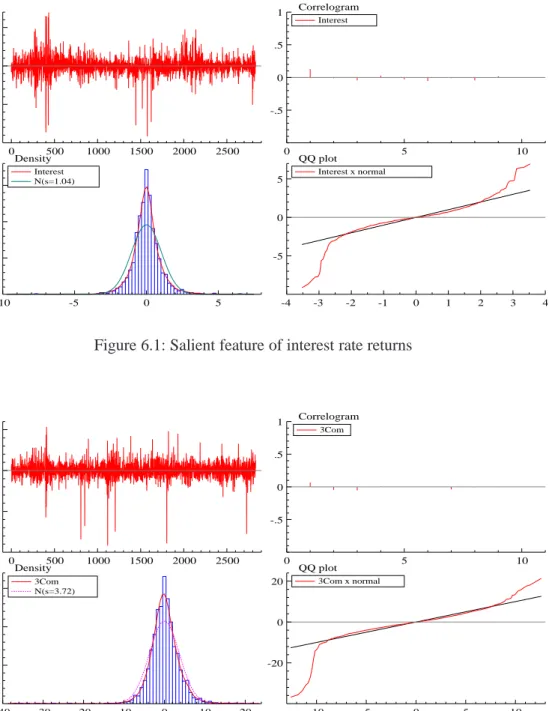
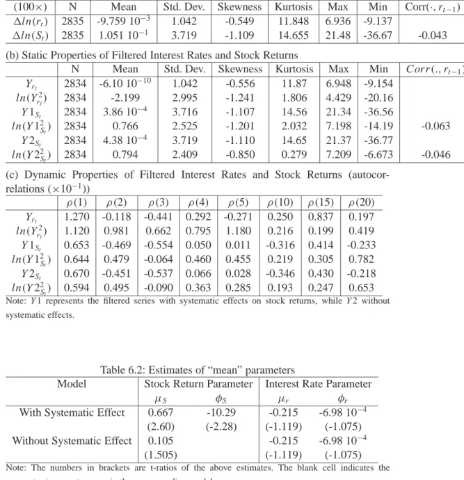
Summary statistics of both interest rates and stock returns are reported in Table 6.1, a time-series plot and salient features of both data sets can be found in Figures 6.1 and 6.2. The interest rates used in this paper as a proxy of the riskless rates are daily U.S. 3-month Treasury bill rates and the underlying stock considered in this paper is 3Com Corporation which is listed in NASDAQ. Both the stock and its options are actively traded. The stock claims no dividend and thus theoretically all options on the stock can be valued as European type options. The data covers the period from March 12, 1986 to August 18, 1997 providing 2,860 observations. From Table 6.1, we can see that both the first difference of logarithmic interest rates and that of logarithmic stock prices (i.e. the daily stock returns) are skewed to the left and have positive excess

kurtosis (>>3) suggesting skewed and fat-tailed distributions. Similarly, the filtered interest ratesYrt as well as the filtered stock returnsY1st (with systematic effect) and

Y2st (without systematic effect) are also skewed to the left and have positive excess

kurtosis. However, the logarithmic squared filtered series, as proxy of the logarith-mic conditional volatility, all have negative excess kurtosis and appear to justify the Gaussian noise specified in the volatility process. As far as dynamic properties, the filtered interest rates and stock returns as well as logarithmic squared filtered series are all temporally correlated. For the logarithmic squared filtered series, the first order autocorrelations are in general low, but higher order autocorrelations are of similar magnitudes as the first order autocorrelations. This would suggest that all series are roughly ARMA(1,1)or equivalently AR(1)with measurement error, which is con-sistent with the first order autoregressive SV model specification. Estimates of trend parameters in the general model are reported in Table 6.2. For stock returns, interest rate has significant explanatory power, suggesting the presence of systematic effect or certain predictability of stock returns. For logarithmic interest rates, there is an insignificant linear mean-reversion, which is consistent with many findings in the literature.

Since the score-generator should give a good description of the data, we further look at the data through specification of the score generator or auxiliary model. We use the score-generator as a guide for the structural model, as there is a clear relationship between the parameters of the auxiliary model and the structural model. If some aux-iliary parameters in the score-generator are not significantly different form zero, we set the corresponding structural parameters in the SV modela priori equal to zero. Various model selection criteria and t-statistics of individual parameters of a wide variety of different auxiliary models that were proposed in Section 3 indicate that (i) Multivariate M-EGARCH(1,1) models are all clearly rejected on basis of the model selection criteria and thet–values of the parameterδ.We therefore set the correspond-ing SV parameterλ1a priori equal to zero. Through (10) this impliesλ4=0; (ii) The

parameterπwas marginally significant at a 5% level. On basis of the BIC, however, inclusion of this parameter is not justified. This rejects that the short-term interest rate is correlated with conditional volatility of the stock returns. A direct explanation of this finding is that either the volatility of the stock returns truly does not have a systematic component or the short-term interest rate serves as a poor proxy of the systematic factor. We believe the latter conjecture to be true as we re-ran the model with other stock returns and invariably foundπ insignificantly different from zero. We therefore set its corresponding parameterα a priori equal to zero; (iii) The cross termsγ12,1andγ21,1were significantly different from zero albeit small, again on

ba-sis of the BIC inclusion of these parameters was not justified. Therefore we included no cross terms between lnσ2

suitable order for the Hermite polynomial in the SNP expansion, we observe that for all modelsKxshould be equal to zero, and, more importantly, according to the most conservative criterion, i.e. the BIC,Kz > 10.This is undesirable. For the choice of the size ofKz, our argument is as follows. The results in van der Sluis (1998) which studied the cases with sample sizes 1,000 and 1,500 indicate that, for these sample sizes,Kz of 4 or 5 was found to be BIC optimal. For our sample which consists of about 3,000 observations, the BIC is in favor of Hermite polynomials of order Kz larger than 10. However, recent results in Andersen, Chung and Sørensen (1997) and van der Sluis (1998) suggest that for sample sizes of 3,000, convergence problems occur in a substantial number of cases for such high order polynomials and that un-der the null of a Gaussian SV model, setting Kz = 0 will yield virtually efficient EMM estimates, which are not necessarily dominated by settingKz >0.

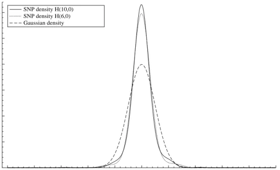
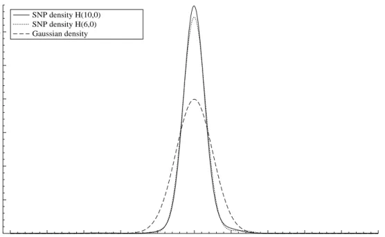
Still we can learn something from the fitted SNP densities with Kz > 0. Consider the conditional density implied by the ML estimates for Kz = 6 and 10 for both data sets in Figures 6.4 and 6.5. Clearly, there is evidence in the data that aGaussian EGARCH model is not good enough as was also indicated by model selection criteria and a Likelihood Ratio test. It also appears that forKz > 6 the SNP density starts to put probability mass at outliers. For descriptive purposes such high orders in the auxiliary model can be desirable, however, since under the null of Gaussian SV we cannot get such outliers, there is no need to consider these. Therefore we decided for these sample sizes to set the Hermite polynomial equal to zero. To check the validity of this argument we performed EMM estimation using the EGARCH-H(6,0) as well to see whether the results would differ from the ones with EGARCH-H(0,0), and it turns out that the parameter estimates differ only slightly. However the values of the individual components of theJ test corresponding to the parameters of the Hermite polynomial cause rejection of the SV model by the J test. Further research should therefore include this fact by using a structural model with fatter-tailed noise or jump component. However, such a non-Gaussian SV model will make option pricing much more complicated, and we leave it for future research. The conclusion is that a Gaus-sian SV model may not be adequate and one should consider a fatter-tailed SV model or ajump process. This can also be seen by comparing the sample properties of the data with the sample properties of the SV model in the optimum.

4.2 Structural models and Estimation Results

The general model: the model specified in Section 2.1 assumes stochastic volatility for both the stock returns and interest rate dynamics as well as systematic effect on stock returns. This model nests the Amin and Ng (1993) model as a special case when

• Submodel 1: No systematic effect, i.e. φs = 0 and α = 0, i.e. a bi-variate stochastic volatility model;

• Submodel 2: No stochastic interest rates, i.e. interest rate is constant,rt =r, which is the Hull-White model and the Bailey and Stulz (1989) model; • Submodel 3: Constant stock return volatility but stochastic interest rate,σst =

σ, which is the Merton (1973), Turnbull and Milne (1991) and Amin and Jarrow (1992) models;

• Submodel 4: Constant stock return volatility and constant interest rate,σst =

σ, rt =r, which is the Black-Scholes model.

The results reported here are all forKx =0 andKz =0. As said in Section 4.1 the models have also been estimated settingKz =6 but no substantial differences were found in the estimation results.

• General model: The estimates for the mean terms are given in Table 6.2. We obtained the following estimates for the symmetric SV model using the EGARCH(1,1)-H(0,0) score generator withκ2=0,

yt =σtt lnσ2 t+1= .005 + .955 lnσ 2 t+ .218 ηt (.065) (30.1) (16.2)

for the interest rates and

yt =σtt lnσ2 t+1= .161 + .940 lnσ 2 t+ .161 ηt (30.8) (66.1) (17.5)

for the stock prices. In order to obtain the filtered series, we used an au-toregressive model with 34 lags for the interest rate and an auau-toregressive model with 29 lags for the stock prices. For the asymmetric model we use the EGARCH(1,1)-H(0,0) as a score generator to obtain the following estimates

yt =σtt

lnσ_t2₊₁= .004 + .959 lnσt2+ .222 ηt

(.107) (47.4) (31.8)

Cor(t, ηt)= −.270

(−156)

for the interest rates and

yt =σtt lnσ2 t+1= .175 + .935 lnσt2+ .161 ηt (121) (233) (35.2) Cor(t, ηt)= −.424 (−164)

for the stock prices.

It is noted that similar to other financial time series, the persistence parameter is close to unity. The asymmetry is moderate for both series and significantly different from zero. The leverage effect is somewhat higher for the stock returns than for the interest rate changes. For the purpose of reprojection, we incorporate asymmetry and the AIC advocates to use 31 lagged lny_t2and 20 laggedztfor interest rates and 28 lagged lnyt2 and 28 laggedzt for stock returns. The filtered series for the stock returns using the symmetric and asymmetric models are displayed in Figure 6.6. Filtered series for the interest rates are displayed in Figure 6.7.

• Submodel 1: The mean terms are given in 6.2. We obtained the following estimates for the symmetric SV model using the EGARCH(1,1)-H(0,0) score generator withκ2=0,

yt =σtt

lnσ_t2= .004 + .959 lnσ_t2₋₁+ .217 ηt

(0.094) (51.8) (31.3)

for the interest rates and

yt =σtt

lnσ_t2= .149 + .944 lnσ_t2₋₁+ .148 ηt

(83.5) (192) (31.3)

for the stock prices. In order to obtain the filtered series, we used an autore-gressive model with 34 lags for the interest rate and an autoreautore-gressive model with 29 lags for the stock prices. For the asymmetric model we used the EGARCH(1,1)-H(0,0) as a score generator to obtain the following estimates

yt =σtt

lnσ_t2₊₁= .004 + .959 lnσ_t2+ .223 ηt

(0.110) (47.8) (31.9)

Cor(t, ηt)= −.275

(−158)

for the interest rates and

yt =σtt

lnσ_t2₊₁= .154 + .944 lnσt2+ .147 ηt

(86.6) (186) (25.4)

Cor(t, ηt)= −.557

(−247)

for the stock prices. The estimates do not differ much from the ones obtained for the general model. For the reprojection we incorporated the asymmetry and the AIC advocates to use 31 lagged lny2

lny2

t and 28 lagged zt for the stock prices. To save space, the filtered series for the submodel have not been displayed. The series resemble the series for the general model very much as displayed in Figures 6.6 and 6.7.

• Other Submodels: Estimation of other submodels is fairly straightforward. Submodel 2 takes the SV part of the stock returns. Submodel 3 takes the SV part of the interest rates.

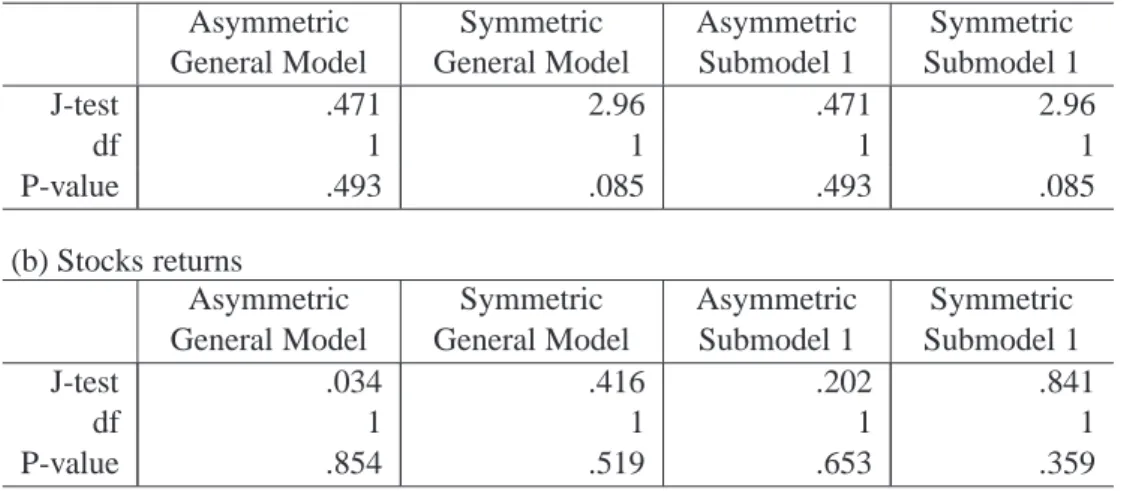
Table 6.3 reports the results of HansenJ-test using EMM. As we see all the models have been accepted at a 5% level. Although aP-value is a monotone function of the actual evidence againstH0,it is very dangerous to choose the best model of these

specifications on basis of theP-values (see Berger and Delampady (1987)). A LR test of the asymmetric SV model versus the symmetric SV model cannot be deduced from the difference in criterion values, since the criterion values are based on different moment conditions, i.e. an EGARCH(1,1)-H(0,0) and an EGARCH(1,1)-H(0,0) with

κ2 =0.However from thet−values corresponding to the asymmetry parameter we

can deduce that the null hypothesis of symmetry will certainly be rejected in favor of the alternative asymmetric model. For submodel 1 we obtain similar results.

For theJ-test with one degree of freedom it is not useful to consider the individual components of the test statistic as in (23). In this case the individual t−values are all about the same. This is a consequence of the fact that the individualt−values are asymptotically equal with probability one in case of only one degree of freedom in the test. As noted in Section 4.1 aJ-test from the EGARCH(1,1)-H(6,0) model leads to rejection of all Gaussian SV models. By inspection of the individual components of the J test we find that in this case the rejection can completely be attributed to the Hermite polynomial. This essentially means that the Gaussian SV model cannot account for the error structure beyond the EGARCH structure that is imposed by the Hermite polynomials. As noted before, a possible solution is to consider non-Gaussian SV models or SV models with jump, but this will not be pursued here.

5. Pricing of Stock Options

The effects of SV on option prices have been examined by simulation studies in e.g. Hull and White (1987), Johnson and Shanno (1987), Bailey and Stulz (1989), Stein and Stein (1991), Heston (1993) as well as empirical studies in e.g. Scott (1987), Wiggins (1987), Chesney and Scott (1989), Melino and Turnbull (1990), and Bak-shi, Cao and Chen (1997). In this paper we will investigate the implications of model specification on option prices through direct comparison with observed market option

prices, with the Black-Scholes model as a benchmark. It is documented in the liter-ature that the Black-Scholes model generates systematic biases in pricing options, with respect to the call option’s exercise prices, its time to expiration, and the un-derlying common stock’s volatility. Since there is a one-to-one relationship between volatility and option price through the Black-Scholes formula, the volatility is of-ten used to quote the value of an option. An equivalent measure for the mispricing of Black-Scholes model is thus the implied or implicit volatility, i.e. the volatility which generates the corresponding option price. The Black-Scholes model imposes a flat term structure of volatility, i.e. the volatility is constant across both maturity and strike prices of options. Thus the use of implied volatility as the measure of pricing errors is less sensitive to the maturity and moneyness of options.

5.1 Description of the Option Data

The sample of market option quotes covers the period of June 19, 1997 through Au-gust 18, 1997, which overlaps with the last part of the sample of stock returns. Since we do not rely solely on option prices to obtain the parameter estimates through fit-ting the option pricing formula, such a sample size is adequate for our comparison purpose. The intradaily bid-ask quotes for the stock options are extracted from the CBOE database. To ease computational burden, for each business day in the sample only one reported bid-ask quote during the last half hour of the trading session (i.e. between 3:30 – 4:00 PM Eastern standard time) of each option contract is used in the empirical test. The main considerations for the choice of the particular bid-ask quote include: i) The movements of stock price is relatively stable around the point of time so that the option quotes are well adjusted; ii) Option quotes which do not satisfy arbitrage restrictions are excluded. The stock prices are calculated as average of bid-ask quotes which are simultaneously observed as the option’s bid-ask quote. Therefore they are not transaction data and the data set used in this study avoids the issue of non-synchronous prices.

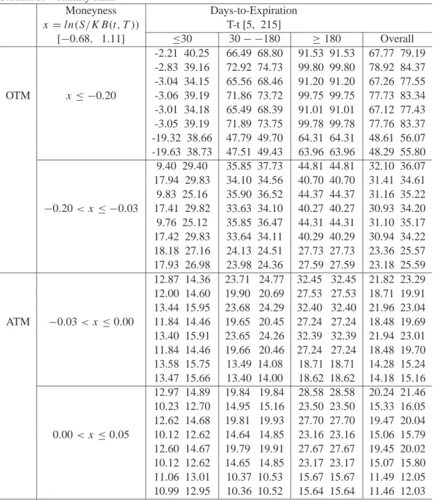
The sampling properties of the option data set are reported in Table 6.4. The data only include options with at least 5 days to expiration to reduce biases induced by liquidity-related issues. We divide the option data into several categories according to either moneyness or time to expiration. In this paper, we use a slight different definition of moneyness for options from the conventional one3_{. Following Ghysels,}

3 In practice, it is more common to call an option as at-the-money/in-the-money/out-of-the-money whenSt = K/St > K/St < K respectively. For American type options with possibility of early exercise, it is more convenient to compareSt withK, while for European type options and from an economic point of view, it is more appealing to compareStwith the present value of the strike priceK.

Harvey and Renault (1996), we define

xt =ln(St/Ke−

RT

t rτdτ) (30)

Technically ifxt =0, the current stock priceSt coincides with the present value of the strike priceK, the option is called at-the-money; ifxt >0 (respectivelyxt <0), the option is called in-the-money (respectively out-of-the-money). In our partition, a call option is said to be at-the-money (ATM) if−0.03 < x ≤ 0.05; out-of-the-money (OTM) ifx ≤ −0.03; andin-the-money (ITM) ifx >0.05. A finer partition resulted in six moneyness categories as in Table 6.4. According to the time to expi-ration, an option contract can be classified as: i) short-term (T −t ≤ 30 days); ii) medium-term (30 < T −t < 180 days); and iii) long-term (T −t ≥ 180 days). The partition according to moneyness and maturity results in 18 categories as in Ta-ble 6.4. For each category, the average bid-ask midpoint price and its standard error, the average effective bid-ask spread (i.e. the ask price minus the bid-ask midpoint) and its standard deviation, as well as the number of observations in the category are reported. Note that among 2120 total observations, about 26.56% are OTM options, 12.69% are ATM options, 60.75% are ITM options; 26.23% are short-term options, 49.01% are medium-term options, and 24.76% are long-term options. The average price ranges from $0.223 for short-term deep out-of-the-money options to $25.93 for long-term deep in-the-money options, and the average effective bid-ask spread ranges from $0.066 for short-term deep out-of-the-money options to $0.375 for log-term deep in-the-money options.

Figure 6.8 plots the implied Black-Scholes volatility against moneyness for options with different terms of maturity. The implied Black-Scholes volatilities are backed out from each option quote using the corresponding stock price, time to expiration, and the current yield of U.S. treasury instruments with maturity closest to the ma-turity of the option. Namely, we use 3-month T-bill rates for options with mama-turity less than 4 months, and 6-month T-bill rates for options with maturity longer than 4 months. The yields are hand-collected from theWall Street Journal over the sample period and the discount rates are converted to annualized compound rates. It is noted that the Black-Scholes implied volatility exhibits obvious U-shaped patterns (smiles) as the call option goes from deep OTM to ATM and then to deep ITM, with the deep-est ITM call option implied volatilities taking the highdeep-est values. The volatility smiles are more pronounced and more sensitive to the term to expiration for short-term op-tions than for the medium-term and long-term opop-tions. Furthermore, the volatility smiles are obviously skewed to the left, indicating a downside risk anticipated by option traders. These observations indicate that the short-term options are the mostly severely mispriced ones by the Black-Scholes model and present perhaps the greatest challenge to any alternative option pricing model. The asymmetry, however, indicates

a possible skewness due to such as the leverage effect or a negative random jump is expected by the option traders on the dynamics of stock returns. These findings of clear moneyness- and maturity-related biases associated with the Black-Scholes model are consistent with the findings for many other securities in the literature (see e.g. Rubinstein (1985), Clewlow and Xu (1993), Taylor and Xu (1993)).

5.2 Testing Option Pricing Models

As Bates (1996b) points out, fundamental to testing option pricing models against time series data is the issue of identifying the relationship between thetrue process followed by the underlying state variables in the objective measure and the “risk-neutral” processes implied through option prices in an artificial measure. Represen-tative agent equilibrium models such as Rubinstein (1976), Brennan (1979), Bates (1988, 1991), and Amin and Ng (1993) among others indicate that European options that pay off only at maturity are priced as if investors priced options at their expected discounted payoffs under an equivalent “risk-neutral” representation that incorporates the appropriate compensation for systematic asset, volatility, interest rate, or jump risk. Thus, the corresponding “risk-neutral” specification of the general model spec-ified in Section 2 involves compensation for various factor risk. Namely, the “mean” of stock return in the “risk-neutral” specification will be equal to the risk-free rate, the “mean” of the interest rate process as well as the “means” of the stochastic con-ditional volatilities for both interest rate and stock return will be adjusted for the interest rate risk and systematic volatility risk. Standard approaches for pricing sys-tematic volatility risk, interest rate risk, and jump risk have typically involved either assuming the risk is nonsystematic and therefore has zero premium, or by imposing a tractable functional form on the risk premium (e.g. the factor risk premiums are pro-portional to the respective factors) with extra (free) parameters to be estimated from observed options prices or bond prices (for interest rate risk).

Under the “risk-neutral” distribution of the general framework, a European call op-tion on a non-dividend paying stock that pays off max(ST −X,0)at maturityT for exercise priceXis priced as

C0(S0, r0, σr0, σS0;T , X)=E∗0[e− RT

0 rtdt_max(S

T −X,0)|S0, r0, σr0, σS0] (31)

where E∗₀ is the expectation with respect to the “risk-neutral” specification for the state variables conditional on all information att = 0. In particular, when λ2 = 0

in the general model setup, i.e. Assumption 2 of Amin and Ng (1993) is satisfied, the option pricing formula can be derived as in (13). The call option price is the expected Black-Scholes price with the expectation taken with respect to the stochastic variance over the life of the option, i.e. the European call option prices depend on