DIFFERENCE STENCILS FOR PRICING AMERICAN OPTIONS UNDER STOCHASTIC VOLATILITY
KAZUFUMI ITO∗ AND JARI TOIVANEN†
Abstract. The deterministic numerical valuation of American options under Heston’s stochastic volatility model is considered. The prices are given by a linear complementarity problem with a two-dimensional parabolic partial differential operator. A new truncation of the domain is described for small asset values while for large asset values and variance a standard truncation is used. The finite difference discretization is constructed by numerically solving quadratic optimization problem aiming to minimize the truncation error at each grid point. A Lagrange approach is used to treat the linear complementarity problems. Numerical examples demonstrate the accuracy and effectiveness of the proposed approach.
Key words.American option pricing, stochastic volatility model, linear complementarity prob-lem, finite difference method, quadratic programming, multigrid method, Lagrange method, penalty method
AMS subject classifications. 35K85, 65M06, 65M55, 65Y20, 91B28
1. Introduction. The seminal papers [2] and [28] by Black & Scholes, and Mer-ton, respectively, laid the foundations of the modern theory of pricing financial op-tions. Since then vast body of scientific work has been devoted to the development of methods for pricing options. Particularly American options are challenging to evalu-ate due to their early exercise possibility and various approaches to approximevalu-ate their price have been proposed. The paper [4] by Brennan and Schwartz was one of first ones to formulate a linear complementarity problem (LCP) and then to solve it using a finite difference discretization. Empirical evidence has shown that the assumption on log-normal behavior of the value of the underlying asset is not realistic for many asset categories including shares of companies. To alleviate this, many generalizations have been introduced for the log-normal model. We consider stochastic volatility models which assume that the volatility of the value of the asset follows a stochastic process; see [11] and references therein. Particularly, our model problem for American options is based on Heston’s model [14], but the techniques considered in this paper can be generalized also for other stochastic volatility models like the Hull-White model [17] and the Stein-Stein model [33].
Based on Heston’s stochastic volatility model, a LCP with a parabolic partial differential operator can derived for the price of American options with the value of underlying asset and its variance being the spatial variables. Near the axes, the first-order derivatives dominate the second-order derivatives in the operator. It also includes the second-order cross derivative. Due to these properties, it is not easy to construct an accurate and stable discretization. In financial literature, most often finite differences are used for the discretization while sometimes also finite elements are used; see [1], [34], [38], for example. It is desirable to use discretizations leading to matrices with the M-matrix property [39]; see also [41]. This property guarantees the stability of the spatial discretization and the feasibility and monotone property
∗Department of Mathematics, Box 8205, North Carolina State University, Raleigh, NC 27695-8205, USA. ([email protected]).
†Institute for Computational and Mathematical Engineering, Building 500, Stanford University, Stanford, CA 94305, USA, ([email protected]).
of the numerical solutions. Many different solution methods have been proposed for the resulting discrete LCPs; see [8], [9], [21], [29], [40]. While these methods have pronounced impact on the efficiency of the valuation of the option the discretization often has more influence on it. In the following, we describe briefly methods considered in the scientific literature.
Clarke and Parrott apply coordinate transform and then perform the discretiza-tion using finite differences on uniform grids in [8], [9]. Their mainly central finite difference discretization switches the discretization of the first-order derivative to an upwind difference when the central difference could lead to oscillations. They employ constant and adaptive time steps with aθ-scheme using the value ofθmaking it close to the Crank-Nicolson method. The resulting LCPs are solved by a projected full approximation scheme (PFAS) multigrid method [3].
In [40], Zvan, Forsyth, and Vetzal use linear finite elements for discretizing the second-order terms and a finite volume discretization for the first-order terms. Fur-thermore, they use a nonlinear van Leer flux limiter to avoid oscillations. Their grids are nonuniform and adaptive time steps are employed with the Crank-Nicolson method. They consider two penalty methods for LCPs. The arising nonlinear and linear problems are solved using a semismooth Newton method and the BICGSTAB method with an incompleteLU preconditioner, respectively.
Oosterlee uses second-order finite difference discretizations on uniform grids and time integration is performed using the BDF2 method with constant time steps in [29]. The resulting LCPs are solved using the PFAS multigrid method.
In [21], seven point finite difference discretizations are used on nonuniform grids. The discretization is constructed in such a way that an M-matrix is obtained. Due to this, in a part of the domain the discretization is only first-order accurate. The time discretizations are based on the Rannacher scheme [31] with constant time steps. Moreover, in [21], the projected SOR method, a projected multigrid method [32], an operator splitting method [18], [19] with a multigrid, a penalty method [40] with a multigrid, and an componentwise splitting method [20] are compared.
In this paper, we consider techniques to improve the efficiency of the computa-tion of the price of opcomputa-tions. Under Heston’s model the first-order derivative terms dominates the second-order derivative terms for small asset values. In this part of the domain, a fine grid is required in order to construct a stable discretization leading an M-matrix. Here we prove that the asset values can be truncated to (Xmin,∞) with-out effecting the prices of American options. This way one can remove fine grid for small asset values and significantly improve the computational efficiency. We propose effective choices for the lower bound Xmin >0 in Section 3. For large asset values and variances a nonuniform grid can be made coarse without increasing error. With such a grid the location of the truncation boundary can be chosen to be fairly far without essentially increasing computational work.
solved fast and the resulting discretization leads to very good accuracy. Earlier such an optimization approach has been used to construct stencils for constant coefficient operators near an interface in [26] and its follow-up papers. It is a novel idea to use this approach for varying coefficient operators in the whole computational domain and not just near boundary/interface.
We solve the resulting LCPs using a Lagrange multiplier method [15], [22]; see also [1]. With a suitable choice of parameters (see ¯λin (5.2)), this method leads to option prices which always satisfy the early exercise constraint, that is, the prices are arbitrage free in this sense. For the option pricing a penalty method considered in [10] and [40] is also obtained from the Lagrange multiplier method with a trivial choice of the parameters. The penalty method leads to small violations of the early exercise constraint. The numerical experiments show that the Lagrange multiplier method and the penalty method are very similar with respect to the accuracy and computational effort. In [22] an error estimate of the proposed method is obtained. The method uses the semi-smooth Newton [23] and it becomes standard for solving nonsmooth equations. In addition, we refer to [6], [25], [36] and references therein for the theory and applications of the semi-smooth Newton method.
The outline of the paper is the following. Section 2 describes a model LCP obtained from Heston’s stochastic volatility model for American put options. The truncation of the computational domain is considered in Section 3. The optimization approach to construct finite difference stencils and time discretization are described in Section 4. Section 5 considers a Lagrange multiplier approach for solving the discrete LCPs. Numerical experiments are presented in Section 6 and the paper ends with conclusions.
2. Model problem. In this section, we describe a linear complementarity prob-lem (LCP) for pricing American put options. Under Heston’s stochastic volatility model and with suitable assumptions on the markets a LCP with a two-dimensional parabolic partial differential operator can be derived for the price of American op-tions; see [14], [38], [40]. In general, these LCPs need to solved numerically; see, for example, [9], [16], [29], [30], [40].
We denote the price of the option byv, the time byt, the price of the underlying asset byx, and its variance byy. Heston’s model leads to a spatial operator
Av =−12y x2vxx−ργy x vxy−12γ2y vyy−r x vx−(α(β−y)−ϑγ√y)vy+r v, (2.1)
where theris the risk free interest rate,β is the mean level of the variance, αis the rate of reversion on the mean level, andγis the volatility of the variance. The market price of the riskϑis assumed to be zero in the rest of the paper similarly to [9], [29], [40]. The correlation between the price of the underlying asset and its variance isρ.
The price at the exercise moment is given by the payoff functionψ. Furthermore, it also defines a final condition
v(x, y, T) =ψ(x). (2.2)
For a put option with the exercise priceK, the payoff function is
ψ(x) = max{K−x,0}. (2.3)
v(x, y, t)≥ψ(x). In the region where the constraint is inactive the pricev satisfies a partial differential equation d
dtv−Av = 0. By combining these relations, a time
dependent linear complementarity problem is obtained for the price of the American option. It is not know a priori where the constraint is active and this makes deriving analytical formulas for the price intractable.
The linear complementarity problem (LCP) for the price of the American put option is
d
dtv(x, y, t)−Av≥0 ⊥ v(x, y, t)≥ψ(x) (2.4)
in a domain {(x, y, t)| x >0, y >0, t∈(0, T)} with the final condition (2.2). The symbol ⊥ indicates that both inequalities are satisfied with at least one of them is holding as equality a.e. On the boundaries x = 0 and y = 0, Dirichlet boundary conditions
v(0, y, t) =ψ(0) and v(x,0, t) =ψ(x) (2.5)
are posed. On far-field the asymptotic behavior ofv satisfies the conditions
lim
x→∞vx(x, y, t) = 0 and ylim→∞vy(x, y, t) = 0. (2.6) These conditions are described in [9] and [29], for example.
It is more customary to solve forward problems in time than backward ones. For this reason, we revert the time by defining a price function uto be u(x, y, t) =
v(x, y, T−t) and considering the solution ofuinstead ofv. The price usatisfies the LCP
d
dtu+Au≥0 ⊥ u≥ψ (2.7)
in the domain{(x, y, t)|x >0, y >0, t∈(0, T)} with an initial condition
u(x, y,0) =ψ(x). (2.8)
The boundary conditions are obtained from (2.5) and (2.6) by replacingv byu. 3. Truncation of domain.
3.1. Upper truncation boundary for y. We start by truncating the
infi-nite computational domain in the direction of variance y. For this purpose, we choose sufficiently large value Y. Then then the LCP (2.7) is posed in the domain {(x, y, t)|x >0, y ∈(0, Y), t∈(0, T)}with the boundary condition
uy= 0 on (0,∞)× {Y}. (3.1)
Based on numerical studies it has been observed thatY should be, say, from four to six times larger than the value of the variance of interest in order to obtain prices with sufficient accuracy for practical purposes [9], [29], [40].
3.2. Black-Scholes model for American options. In order to derive a lower truncation boundary forx, we start by considering the one-dimensional Black-Scholes model for American options given by a LCP of the form
d
dtvˆ(x, t) +
1 2σ
2x2vxxˆ +rxvxˆ
−rvˆ≤0 ⊥ vˆ(x, t)≥ψ(x)
ˆ
v(x, T) =ψ(x)
a.e. (x, t)∈(0,∞)×(0, T). The volatility of the asset price is σ >0. The comple-mentarity system (3.2) has the following interpretation in mathematical finance. The price processXtis governed by the Ito’s stochastic differential equation:
dXt=rXtdt+σStdBt, (3.3)
or
XT = exp
µµ r−1
2σ 2
¶
(T−t) +σ(BT −Bt)
¶
Xt (3.4)
where Bt denotes the standard Brownian motion and the value function ˆv is repre-sented by
ˆ
v(x, t) = sup
τ
Ex,the−r(τ−t)ψ(Xτ)i over all stopping times t≤τ≤T. (3.5)
It can be easily shown from this that ˆv(x, t) is monotonically nonincreasing in both
x >0 and t < T.
To express (3.2) in variational form we define
a(ˆv, φ) =
Z ∞
Xmin µµ
1 2σ
2x2ˆvx+ (r
−σ2)xˆv ¶
φx+ (2r−σ2)ˆvφ ¶
dx (3.6)
for ˆv, φ∈V, whereV is the completion of the space
½
φ∈H |φis absolutely continuous on (Xmin,∞),
Z ∞
Xmin
x2|φx|2dx <∞ and φ(x)→0 as x→ ∞ and x→Xmin
¾ (3.7)
under the norm
|φ|2V = Z ∞
¯
X
(x2|φx|2+|φ|2)dx. (3.8)
The solution to (3.2) satisfies ˆv−ψ∈V. Setting ˆu(x, t) = ˆv(x, T−t)−ψwe arrive at
¿ d
dtuˆ(t), w−uˆ(t) À
+a(ˆu(t), w−uˆ(t))−a(ψ, w−uˆ(t))≥0 for allw∈ C,
ˆ
u(x,0) = 0,
(3.9)
whereC ={w∈V |w≥0}. Here, we can choose the interval on which the solution ˆ
v is defined, as (Xmin,∞),Xmin>0 and it allows to avoid the singularity at 0. The LCP (3.2) has the equilibrium solution of the form
¯
v(x) =
K−x, x≤Xmin,
(K−Xmin)³ x Xmin
´−γ
, x≥Xmin,
(3.10)
where
Xmin=
Kκ
1 +κ and κ=
2r
The equilibrium solution satisfies the Cauchy-Euler equation 1
2σ
2x2vxxˆ +r xvxˆ −rvˆ= 0 in (X
min,∞). (3.12) Thus, it can be expressed as
ˆ
v(x) =C1xs1+C2xs2, (3.13)
wheres1=−κands2= 1 satisfy 1
2σ 2s(s
−1) +r s−r=
µ
1 2σ
2s+r
¶
(s−1) = 0. (3.14)
Since ˆv→0 asx→ ∞, we have ˆv=C1x−κ. As ˆv∈H2(0,∞) [22] we must have
ˆ
v(Xmin) =K−Xmin, vxˆ (Xmin) = (K−Xmin) −
κ Xmin
=−1, (3.15)
which yields (3.10). Since ˆv is monotone in t, ˆv(x, t) ≤ ¯v(x) for all t ≤ T and ˆ
v(x, t)→v¯(x) monotonically ast→ −∞for allx≥0. This validates our claim. 3.3. Lower truncation boundary for x. The corresponding bilinear form a
forAdefined by (2.1) is given by
a(u, φ) =
Z µ1
2yx
2uxφx+ (yx
−r)uxφ+ruφ
+1
2(ργ(vxφy+vyφx) +γ
2yvyφy)
−ργ2 (xvxφ+yvyφ) + (γ2−α(β−y))vyφ ¶
dx
(3.16) foru, φ∈H1. Thus, ifu+= sup{u,0} ∈H1, then
a(u, u+)≥
Z µ1
−ρ
2 (yx 2
|u+x|2+γ2y|u+y|2) +
1
2(3r−y−ργ−γ 2
−α)|u+|2
¶ dx.
(3.17) Thus, it can be shown as in [22] that (2.7) has a solution u ∈ H1
loc(0, T;L2)∩ L2
loc(0, T;H2) and thatu(·, t) is monotonically nondecreasing in t. Let
˜
u(x, y) = ¯v(x) (3.18)
anduis the steady state solution to (2.7), i.e. satisfies
Au≥0 ⊥ u≥ψ a.e. (3.19)
Then, the following theorem shows that the boundary value problemv(Xmin, y, t) =
ψ(Xmin) at the truncated boundaryx=Xmin provides the exact solution to (2.4). Theorem 3.1. Let ˜ucorresponds to the steady state v¯ of the one-dimensional model withσ2=Y, whereY is the upper bound ofy. Thenu˜≥u(x, y)andx=Xmin
provides a lower-bound estimate of the active region defined by{u=ψ}. Proof. On{u > ψ} ∩ {u > ψ˜ }
A(˜u−u) =−12(y−σ2)κ(κ+ 1)
µ x Xmin
¶−κ
≥0 (3.20)
and on{u > ψ} ∩ {u˜=ψ}
3.4. Time-dependent lower truncation boundary for x. Let ˜u(x, y, t) =
ˆ
v(x, T −t), where ˆv is the solution of (3.2). That is, ˜uis the solution of the one-dimensional LCP
d
dtu˜(x, y, t)−
1 2σ
2x2uxx˜
−rx˜ux+r˜u≤0 ⊥ u˜(x, y, t)≥ψ(x) (3.22)
with ˜u(x, y,0) =ψ(x). The following theorem shows that a lower-bound estimate can be also obtained from the one-dimensional model (3.22) withσ2=Y.
Theorem 3.2. It holds that u˜(·, t) ≥ u(·, t) a.e. and, thus, the free surface S(t) =∂{u˜(x, t)> ψ(x)} ∈(0, K)determined by the one-dimensional equation (3.22)
withσ2=Y provides a lower bound estimate for the one for (2.7).
Proof. Since ˜ux≤0 and d
dtu˜ ≥0 a.e., ˜uxx≥0 holds a.e.. Furthermore, ˜uy = 0.
Thus, on{u > ψ} ∩ {u > ψ˜ }
d
dt(˜u−u) =−A(˜u−u) +
1 2(σ
2
−y)˜uxx (3.23)
and on{u > ψ} ∩ {u˜=ψ}
d
dt(˜u−u) =−A(˜u−u) +rK. (3.24)
Let Ωt= ©
(x, y)T |u(x, y, t)> ψ(x)ªandφ= inf{u˜−u,0} ∈H1(0, T;L2). Then for
ω≥0
d dt
Z
Ωt
1 2e
−ωt
|φ|2dx=e−ωt(
Z
Ωt
(φd
dt(˜u−u)−ω|φ|
2)dx+
Z
Γt
1 2|φ|
2(h
·n)ds) (3.25)
where n=∇u/|∇u|and his the velocity of the interface Γt=∂Ωt. Since φ= 0 at
Γt and from (3.17) and (3.23)–(3.24) Z
Ωt
φd
dt(˜u−u)−ω|φ|
2dx ≤ −
Z
Ωt
((A(˜(u)−u), φ) +ω|φ|2)dx≤0.
It thus follows from (3.23)–(3.25) that
d dt
Z
Ωt
1 2e
−ωt
|inf{u˜−u,0}|2dx≤0 (3.26)
and thus ˜u≥ua.e.
3.5. Upper truncation boundary for x. For the one-dimensional
Black-Scholes model as well as for its multidimensional generalizations the truncation error has been studied in [24] when a Dirichlet boundary condition is posed on the trunca-tion boundary. They conclude that the usual rule of thumb to truncate at three or four times the exercise price is usually sufficient. Based on numerical studies [9], [29], [40], for Heston’s model with the homogenous Neumann boundary condition posed on the truncation boundary two or three times exercise price seems to be sufficient. We denote the location of the truncation boundary byXmaxand the Neumann boundary condition posed on it is given by
4. Discretization. For the computational domain [Xmin, Xmax]×[0, Y]×[0, T], we define a space-time grid
(xi, yj, tk)∈ {x0, . . . , xm} × {y0, . . . , yn} × {t0, . . . , tl}, (4.1)
where xi < xi+1, yj < yj+1, tk < tk+1, x0 =Xmin, xm =Xmax, y0 = 0, yn =Y,
t0= 0, and tl=T.
4.1. Spatial finite difference discretization. The Dth degree Taylor poly-nomial of the two-dimensional function u(x+ ∆xi) atx= (x y)T and the order of
the remainder is given by
u(x+ ∆xi) =u(x) +
M X
k=1
dk,i∂δku(x) +O(k∆xikD+1), (4.2)
whereM = 1
2(D+ 1)(D+ 2)−1 and multi-indicesδ
ks are defined as
δk = (j−k, k+i−j), i= 1 2(
√
9 + 8k−3), j= 1
2(i+ 1)(i+ 2)−1. (4.3) That is, the nine first multi-indicesδk are given by
δ1= (1,0), δ2= (0,1),
δ3= (2,0), δ4= (1,1), δ5= (0,2),
δ6= (3,0), δ7= (2,1), δ8= (1,2), δ9= (0,3).
(4.4)
The coefficientsdk,i in (4.2) are defined as
dk,i= 1 |δk|!
µ
|δk|
δk
2
¶
(∆xi)δk = 1
δk
1!δk2!
(∆xi)δk1(∆yi)δ
k
2. (4.5)
Let us have N grid points x+ ∆xi, i = 1, . . . , N, around x and let the
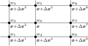
corre-sponding finite difference weights at these points be denoted bywi. Furthermore, let the weight atx be w0 and ∆x0 =0. The standard compact nine point stencil and the notations are shown in Figure 4.1. Then anN+ 1 point finite difference sum has an approximate Taylor polynomial presentation
N X
i=0
wiu(x+ ∆xi)≈
N X
i=0
wiu(x) +
N X i=1 wi M X k=1
dk,i∂δk
u(x)
≈u(x)
N X
i=0
wi+³∂δ1
u(x) · · · ∂δM
u(x)´Dw,
(4.6)
where we have use the notations
D=
d1,1 · · · d1,N
..
. . .. ...
dm,1 · · · dM,N
and w=
w1 .. . wN
. (4.7)
With the finite difference sum (4.6), we approximate the operator
b0u(x) +
M X
k=1
bk∂δk
u(x) =b0u(x) +
³ ∂δ1
u(x) · · · ∂δM
u(x)
´
s x+∆x1
w1
s x+∆x2
w2
s x+∆x3
w3
s x+∆x4
w4
s x w0
s x+∆x5
w5
s x+∆x6
w6
s x+∆x7
w7
s x+∆x8
w8
Fig. 4.1.The standard nine point finite difference stencil atxwith the coordinates of the grid points and the associated weightswi.
where b=¡b1 · · ·bN¢
T
. For example, for the operator A in (2.1), the bis are given by
b0=r, b1=−rx, b2=−α(β−y),
b3=−12yx2, b4=−ργyx, b5=−12γ2y,
(4.9)
and bk = 0, k = 6, . . . , M. By using (4.6) and (4.8), we obtain for the truncation error an estimate
N X
i=0
wiu(x+ ∆xi)−b0u(x)−
M X
k=1
bk∂δku(x)
≈u(x)
à N X
i=0
wi−b0
!
+³∂δ1
u(x) · · · ∂δM
u(x)
´
(Dw−b).
(4.10)
We eliminate the first term in the truncation error (4.10) by choosing the diagonal weight to be
w0=b0−
N X
i=1
wi. (4.11)
There are many ways to choose the other N weights. One approach is to eliminate more terms from the truncation error. This was done in [26] and after this the distance from some given stencil added with a weighted sum of squares of terms in the truncation error was minimized. Our aim is to obtain an M-matrix which means that the weights wi, i = 1, . . . , N, have to be non positive. Due to the varying coefficients of the operator A and the use of nonuniform grids, we do not know a priori how many terms we can eliminate and still obtain an M-matrix.
Our approach is to minimize the truncation error under the non positivity con-straints for the offdiagonal weights. The truncation error depends on partial deriva-tives of u(x) which we do not generally know a priori. In such a case, a natural approach is to minimize weighted squares of their coefficients in the truncation error. By choosing the weights of the squares to be ones, we obtain a least squares problem
min
w≤0kDw−bk
2
2, (4.12)
which yields a finite difference stencil leading to an M-matrix. The problem (4.12) is equivalent with a standard quadratic programming problem (QP)
min
w≤0
1 2w
where Db =DTD andbb =−DTb. This quadratic optimization problem is formed and solved for each grid point. We denote the discretized operatorAby a matrixA. One optimization yields the weightswi, i = 0, . . . , N, and from them the row of A corresponding to the grid point under consideration is assembled.
The partial derivatives appearing in the truncation error can be estimated using an approximation for u which can be computed on fairly coarse grid. This a pos-teriori information can used to choose the weights in the least squares problem for w. This way more optimal finite difference stencils can be constructed. Any a priori information on the relative amplitude of partial derivatives can be used in the same manner.
The spatial discretization of (2.7) leads to a semi-discrete LCP
∂u
∂t +Au≥0 ⊥ u≥ψ, (4.14)
where the vectorsuandψcontain the grid point values ofuandψ, respectively. The symbol ⊥indicates that both inequalities are satisfied componentwise with at least one of them is holding as equality for each component. The initial value ofuis given byψ.
4.2. Temporal discretization. The option pricing model has a nonsmooth initial value. Although the Crank-Nicolson method is popular it does not have good stability properties. In many cases the Crank-Nicolson method can lead to a numerical solution with oscillation because it is not L-stable. In order to obtain numerical solution without undesired oscillations we use the Rannacher time-stepping method [31] in our numerical experiments. This type of method is also applied in the option pricing in [10], [12], [30], for example.
The Rannacher time-stepping scheme performs a few first time steps with the implicit Euler method and after that it uses the Crank-Nicolson method. This way the scheme has good damping properties and second-order accuracy. For the semi-discrete LCP in (4.14) the Rannacher time-stepping scheme reads
¡
I+12∆tbkcA
¢
u(k+1/2)≥u(k) ⊥ u(k+1/2)≥ψ, k= 0,1/2,1,3/2, ¡
I+12∆tkA¢u(k+1)≥¡I−1 2∆tkA
¢
u(k) ⊥ u(k+1)≥ψ, k= 2, . . . , l−1, (4.15) where the time step is ∆tk =tk+1−tk and u(0) = ψ. The implicit Euler method is applied with step sizes ∆t0/2 and ∆t1/2 in the first four time steps and the time-stepping is continued with the Crank-Nicolson method using step size ∆tk, k ≥ 2. The purpose of shorter time steps with the Euler method is to improve accuracy.
The LCPs appearing in the Rannacher time-stepping (4.15) have a general form
Bu≥f ⊥ u≥ψ, (4.16)
where we have omitted indices indicating the dependence on the time step in order to simplify the notations. The matrix Bhas an M-matrix property due to the same property ofA.
5. Lagrange multiplier approach. We adopt the Lagrange multiplier ap-proach proposed in [15] and further considered in [1] and [22] to treat the comple-mentarity conditions. The LCP (4.16) is approximated by
where c is a prescribed positive constant and ¯λ is a given vector with non negative components. The purpose of the term c(ψ−u) is to force the solution towards feasible one. One of the main motivations to include the vector ¯λis that it leads to a feasible solutionuwhen it is chosen according to
¯
λ= max{Bψ−f, 0}. (5.2) The following theorem states this property. An alternative choice ¯λ=0 leads to a penalty method. For pricing American options the penalty method has been consid-ered in [10] and [40], for example.
Theorem 5.1. Let B be an M-matrix and let ¯λ be chosen according to (5.2). Then the solutionuof (5.1) with any non negativecsatisfies the constraintu≥ψ.
Proof. By subtractingBψfrom both side of (5.1), we obtain
B(u−ψ) =f−Bψ+ max©λ¯ +c(ψ−u), 0ª. (5.3) By using the definition of ¯λin (5.2) and rearranging terms, we have
B(u−ψ) = max{max{f−Bψ, 0}+c(ψ−u), f−Bψ}. (5.4) If we havec= 0 then this simplifies to
B(u−ψ) = max{f−Bψ, 0}. (5.5) Due to the non negativity of the right-hand side and the M-matrix property ofB, we haveu−ψ≥0and, thus, we have proven the result for the casec= 0.
In the following, we assume that c > 0. We definev = min{u−ψ, 0}. Then there exists a permutation matrixP such that
˜
v=P v=
µ
˜ u1−ψ˜1
0
¶
and u1˜ −ψ˜1≤0, (5.6)
where ˜u=P u and ˜ψ=P ψ. Then we have
vTB(u−ψ) = ˜vTB˜ ³u˜−ψ˜´
=³u1˜ −ψ˜1
´T
˜
B11³u1˜ −ψ˜1
´
+³u1˜ −ψ˜1
´T
˜
B12³u2˜ −ψ˜2
´ ,
(5.7)
where ˜B=P BPT. The matrix ˜B is an matrix, since it is obtained from an M-matrix by permuting the rows and columns in the same way. Due to this the quadratic term in (5.7) with ˜B11 is non negative. Furthermore,³u1˜ −ψ˜1
´T
and ˜B12 are non positive while ˜u2−ψ˜2 is non negative and, thus, their product which is the term in (5.7) with ˜B12 is non negative. Thus, we have
vTB(u−ψ)≥0. (5.8)
By premultiplying (5.4) withvT and using this inequality, we obtain
LetIbe set of indices defined byI={i|ui <ψi}. Then we have X
i
min{ui−ψi,0}max{max{(f −Bψ)i,0}+c(ψi−ui),(f−Bψ)i}
=X
i∈I
(ui−ψi) max{max{(f −Bψ)i,0}+c(ψi−ui),(f−Bψ)i} ≥0.
(5.10)
For anyi∈I by usingc >0, we obtain
(ui−ψi) max{max{(f−Bψ)i,0}+c(ψi−ui),(f −Bψ)i}
≤ −c(ψi−ui)2<0.
(5.11)
From (5.10) and (5.11), it follows that the setI must be empty and, thus,u≥ψ. The free boundary between the active set{(x, y)|u(x, y) =ψ(x)}and the inactive set{(x, y)|u(x, y)> ψ(x)} can be approximated by
{(x, y)|λ¯(x, y) +c(ψ(x)−u(x, y)) = 0}, (5.12)
whereuand ¯λare interpolated functions defined using the grid point values given by uand ¯λ, respectively. The accuracy of this approximation is at most the order of 1/c; see [22]. This suggest that with a second-order discretization of A a natural choice forcwould be the order of one over grid step size squared.
The problems (5.1) are nonlinear and nonsmooth. Following [40], we employ a semismooth Newton method to solve these problems; see [15] for analysis of this case. The (p+ 1)th iterantup+1is given by
up+1=up+dp, (5.13)
where the vectordp is the solution of the system of linear equations
J(up)dp=f + max©λ¯+c(ψ−up),0ª−Bup=rp. (5.14) The matrix J(up) in (5.14) belongs to the generalized Jacobian [7] at xp and it is
chosen to be
[J(up)]
i,j=Bi,j+ (
c, if i=j and λ¯i+c(ψi−u p i)>0,
0, otherwise. (5.15)
6. Numerical results. The American option pricing problem under stochastic volatility (2.7) is solved with the parameter values
K= 10, T = 0.25, r= 0.1, α= 5, β= 0.16, γ= 0.9, and ρ= 0.1.
For accuracy, it is beneficial to have a finer grid near the strike price K and for small values of volatility. Such a grid is obtained by choosing it according to
xi=Xmin+
µ
1 +sinh(η(i/n−a)) sinh(ηa)
¶
(K−Xmin), i= 0,1, . . . , n, (6.1)
and
yj =
µ
bj/m−1 b−1−1
¶
Y, j= 0,1, . . . , m, (6.2)
where the constantsaandbcontrol the amount of refinement near the strike priceK
and for smally, respectively. The constantηis solved numerically from the equation
xn=Xmax. Similar grid generating functions have been considered in [34], for exam-ple. The price of the put option changes more rapidly close to the expiryT and, thus, it is more efficient to take smaller time steps near the expiry. This is accomplished by choosing the approximation timestk according to
tk =
µdk/l−1
d−1−1
¶
T, k= 0,1, . . . , l, (6.3)
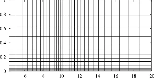
where dis a constant greater than one controlling the refinement. Alternativelytks could be chosen adaptively; see [1], [9], [10]. Based on experiments with different parameters aiming to improve the efficiency, we chose the values a = 0.44, b = 40, andd= 64. Figure 6.1 shows 33×17 grid constructed using the aboveaandb.
0 0.2 0.4 0.6 0.8 1
6 8 10 12 14 16 18 20
Fig. 6.1.The33×17refined space grid.
The following numerical experiments use seven point finite difference stencils which is obtained from the nine point stencils in Figure 4.1 by setting w3 = 0 and
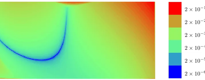
Figure 6.2 shows the seven point stencils without the diagonal weight for the 257×129 grid. From this figure it can be seen that only in a small part of the computational domain some of the weights are zero which corresponds to the red color in the figure. The norm of the vectorsDw−bappearing in (4.12) is shown for the same grid in Figure 6.3. This quantity estimates the truncation error of the finite difference stencil. The prices of options are sought in the middle lower part of the domain and in there the norm is less than 10−3. Moving from there to right and up the norm grows due to coarser grid and larger coefficients in the operatorA. In the following, we present results on the grids: 17×9, 33×17, 65×33, 129×65, 257×129, and 513×257. The maximum values of kDw−bk2 for these grids are: 24.9, 10.1, 3.00, 0.808, 0.209, and 0.0586. Thus, on finer grids the reduction factor of the norm is close to four. With a solution having bounded partial derivatives up to third-order, the reduction factor being four implies second-order accuracy.
-6×10⁻¹
-6×100
-6×101
-6×10²
-6×10³
-6×10⁴
Fig. 6.2.The finite difference stencils for the257×129grid without the diagonal weight. Each pixel in one rectangle corresponds to a grid point and the corresponding pixels in the six rectangles gives the six optimized weights.
2×10⁻¹
2×10⁻²
2×10⁻³
2×10⁻⁴
2×10⁻⁵
2×10⁻⁶
Fig. 6.3.The normkDw−bk2in(4.12)which estimates the truncation error for the257×129
grid with each pixel being a grid point.
see [5], [13], [35], [37].
We start by computing reference prices using a fine grid defined by m = 2048,
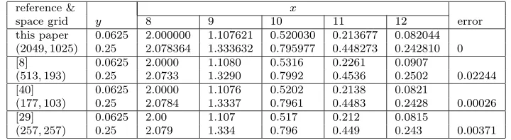
n= 1024, andl= 1024. For this computation, we have used ¯λgiven by (5.2) and fairly strict stopping criteria for the iterative methods. In Table 6.1, the reference prices together with three other sets of prices published in [8], [29], and [40] are reported for the variances 0.0625, 0.25, and for the asset prices 8, 9, 10, 11, 12. Based on the convergence study in the following, we conclude that for the pricing problem in the truncated domain all reference prices have at least five correct decimals. Furthermore, based on experiments not reported here with larger computational domains the error due the truncation from up and right seems to appear in the sixth decimal or later. Thus, we expect that the reference prices have five correct decimals. Based on this, we have computed thel2errors for the price sets and given them in Table 6.1.
Table 6.1
The reference prices, the prices published in scientific literature and their l2 errors based on
the reference prices.
reference & x
space grid y 8 9 10 11 12 error
this paper 0.0625 2.000000 1.107621 0.520030 0.213677 0.082044 (2049,1025) 0.25 2.078364 1.333632 0.795977 0.448273 0.242810 0
[8] 0.0625 2.0000 1.1080 0.5316 0.2261 0.0907
(513,193) 0.25 2.0733 1.3290 0.7992 0.4536 0.2502 0.02244
[40] 0.0625 2.0000 1.1076 0.5202 0.2138 0.0821
(177,103) 0.25 2.0784 1.3337 0.7961 0.4483 0.2428 0.00026
[29] 0.0625 2.00 1.107 0.517 0.212 0.0815
(257,257) 0.25 2.079 1.334 0.796 0.449 0.243 0.00371
For our next experiments, we chose the stopping criterion for the iterative methods to be
krk ≤ 1
10m nkfk, (6.4)
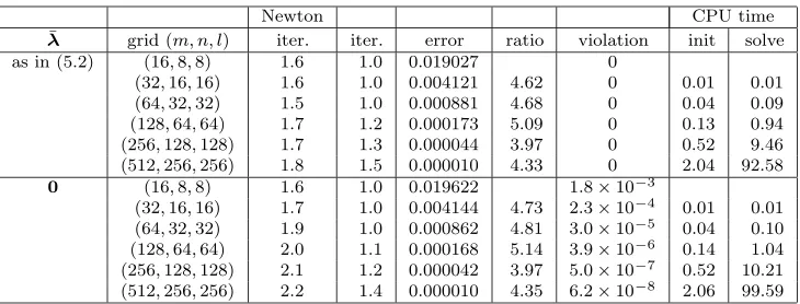
where r is the residual vector andf is the right-hand side vector. The termination of iterations using (6.4) leads to an additional error in the prices which is less than 5%. Table 6.2 reports the results for the six different grids and for two choices for ¯λ in (5.1). The columns of the table gives the average number of Newton and multigrid iterations, the l2 error of the prices based on the reference prices in Table 6.1, the ratios of the consecutive errors, the maximum violation of the constraintu(·, T)≥ψ, and CPU times in seconds on a PC with 3.8 GHz Xeon processor. The column ’init’ gives the time required for forming the matrixA using the QP optimization for the finite difference stencils and ’solve’ gives the time required for the time stepping. For completeness and in order to make future comparisons possible, we have also give the prices for the nonzero ¯λin Table 6.3.
Table 6.2
The average number of iterations, the errors at the ten reference points, the ratios of consecutive errors, the maximum violations of constraint, and the CPU times in seconds for all methods on six grids.
Newton CPU time
¯
λ grid (m, n, l) iter. iter. error ratio violation init solve
as in (5.2) (16,8,8) 1.6 1.0 0.019027 0
(32,16,16) 1.6 1.0 0.004121 4.62 0 0.01 0.01
(64,32,32) 1.5 1.0 0.000881 4.68 0 0.04 0.09
(128,64,64) 1.7 1.2 0.000173 5.09 0 0.13 0.94 (256,128,128) 1.7 1.3 0.000044 3.97 0 0.52 9.46 (512,256,256) 1.8 1.5 0.000010 4.33 0 2.04 92.58
0 (16,8,8) 1.6 1.0 0.019622 1.8×10⁻³
(32,16,16) 1.7 1.0 0.004144 4.73 2.3×10⁻⁴
0.01 0.01 (64,32,32) 1.9 1.0 0.000862 4.81 3.0×10⁻⁵
0.04 0.10 (128,64,64) 2.0 1.1 0.000168 5.14 3.9×10⁻⁶
0.14 1.04 (256,128,128) 2.1 1.2 0.000042 3.97 5.0×10⁻⁷
0.52 10.21 (512,256,256) 2.2 1.4 0.000010 4.35 6.2×10⁻⁸
2.06 99.59
considerable part of the total time only on the coarsest grids while on the finest grid it requires only a couple percent of the time.
The behavior of the solution procedure is fairly similar for both choices of ¯λ. The main difference is that the choice (5.2) satisfies the early exercise constraint as Theorem 5.1 states while ¯λ = 0 leads to small violations which tend to zero as grid is refined. The choice (5.2) leads to a slightly faster convergence of the Newton method while the converse is true for the multigrid method. Thus, the CPU times are essentially the same. Also, the accuracy of both choice is essentially the same under the choicec= (n/Y)2 for the parameterc in (5.1).
We can compare the accuracy of the discretization proposed in this paper and the ones employed in [8], [40], and [29] using Table 6.1 and Table 6.2. The discretization in [8] is the most inaccurate. The finite difference discretization in [29] uses uniform grids without any coordinate transform. This could explain why it is less accurate than the discretization in here and in [40]. The discretization in [40] is fairly accurate. On the (177,103) grid, thel2 error based on the reference prices in Table 6.1 is 2.6×10⁻⁴. With the optimized stencils, we obtained the error 1.7×10⁻⁴ on the (129,65) grid. Thus, the optimized discretization is a couple of times more accurate which is a small difference when compared to the other discretizations. The paper [21] does not report the ten prices, but it does give anl2 error based on different, fairly accurate reference prices. The error in [21] for the componentwise splitting method on the (161,65) grid is 6.2×10⁻³. Thus, the prices in [21] are more than one order of magnitude less accurate than the ones in here and [40] while their accuracy seems to be comparable with the prices in [29]. An essential differences between the optimized discretization in here and the ones in [8], [40], and [29] is that here the M-matrix property is guaranteed while the other discretization usually do not satisfy it. The discretizations in [8] and [29] are fairly easy-to-implement while the ones in here and [40] are more complicated. Thus, there is a clear tradeoff between implementation effort and accuracy.
7. Conclusions. For American put options, we proposed a truncation of a region with small asset values away from the computational domain under Heston’s stochastic volatility model. This makes accurate discretization easier and reduces the number of unknowns in the resulting linear complementarity problems (LCPs).
Table 6.3
The prices computed usingλ¯ in (5.2)and theirl2 errors based on the reference prices.
grid x
(m, n, l) y 8 9 10 11 12 error
(16,8,8) 2.002061 1.098723 0.511742 0.206673 0.079616
2.078986 1.325264 0.788562 0.443066 0.241243 0.019027 (32,16,16) 2.000036 1.105806 0.518176 0.212456 0.081646
2.078813 1.331793 0.794061 0.447137 0.242572 0.004121 (64,32,32) 2.000003 1.107355 0.519686 0.213503 0.081723
2.078608 1.333307 0.795588 0.448095 0.242487 0.000881 (128,64,64) 2.000000 1.107624 0.519987 0.213564 0.081988
2.078387 1.333613 0.795938 0.448189 0.242759 0.000173 (256,128,128) 2.000000 1.107626 0.520021 0.213651 0.082034
2.078383 1.333627 0.795963 0.448252 0.242804 0.000044 (512,256,256) 2.000000 1.107620 0.520026 0.213672 0.082043
2.078358 1.333630 0.795974 0.448270 0.242810 0.000010
fairly complicated operator. The aim of the optimization is to minimize the truncation error when the resulting matrix is required to have the M-matrix property. The numerical results showed that the arising quadratic programming problems can solved much faster than the LCPs with the exception of very coarse grids. We proposed to use a Lagrange multiplier approach to approximate the solutions of LCPs. It can be considered as a generalization of the penalty method described by Zvan, Forsyth, and Vetzal in [40]. With the Lagrange multiplier approach it is possible to guarantee that the prices satisfy the early exercise constraint while the penalty method leads always to small violations.
The numerical results demonstrated that the proposed approach leads to option prices which are more accurate than the prices in the literature. By using a multigrid method proposed by Oosterlee in [29] to solve the resulting systems of linear equations an effective and scalable method to price American options is obtained. The results showed that accurate discretizations are essential for pricing American options under Heston’s model accurately and fast. One possibility to further improve the accuracy of discretizations is to use adaptive grids; see [1], [27], for example.
Acknowledgements. We thank Dr. Samuli Ikonen for many fruitful discussions on numerical methods for option pricing.
REFERENCES
[1] Y. Achdou and O. Pironneau,Computational methods for option pricing, vol. 30 of Frontiers in Applied Mathematics, SIAM, Philadelphia, PA, 2005.
[2] F. Black and M. Scholes,The pricing of options and corporate liabilities, J. Political Econ-omy, 81 (1973), pp. 637–654.
[3] A. Brandt and C. W. Cryer,Multigrid algorithms for the solution of linear complementarity problems arising from free boundary problems, SIAM J. Sci. Statist. Comput., 4 (1983), pp. 655–684.
[4] M. J. Brennan and E. S. Schwartz,The valuation of American put options, J. Finance, 32 (1977), pp. 449–462.
[5] W. L. Briggs, V. E. Henson, and S. F. McCormick,A multigrid tutorial, SIAM, Philadel-phia, PA, second ed., 2000.
[6] X. Chen, Z. Nashed, and L. Qi,Smoothing methods and semismooth methods for nondiffer-entiable operator equations, SIAM J. Numer. Anal., 38 (2000), pp. 1200–1216.
[8] N. Clarke and K. Parrott,The multigrid solution of two-factor American put options, Tech. Rep. 96-16, Oxford Computing Laboratory, Oxford, 1996.
[9] ,Multigrid for American option pricing with stochastic volatility, Appl. Math. Finance, 6 (1999), pp. 177–195.
[10] P. A. Forsyth and K. R. Vetzal,Quadratic convergence for valuing American options using a penalty method, SIAM J. Sci. Comput., 23 (2002), pp. 2095–2122.
[11] J.-P. Fouque, G. Papanicolaou, and K. R. Sircar,Derivatives in financial markets with stochastic volatility, Cambridge University Press, Cambridge, 2000.
[12] M. B. Giles and R. Carter,Convergence analysis of Crank-Nicolson and Rannacher time-marching, J. Comput. Finance, 9 (2006), pp. 89–112.
[13] W. Hackbusch,Multigrid methods and applications, vol. 4 of Springer Series in Computational Mathematics, Springer-Verlag, Berlin, 1985.
[14] S. Heston,A closed-form solution for options with stochastic volatility with applications to bond and currency options, Rev. Financial Stud., 6 (1993), pp. 327–343.
[15] M. Hinterm¨uller, K. Ito, and K. Kunisch,The primal-dual active set strategy as a semis-mooth Newton method, SIAM J. Optim., 13 (2003), pp. 865–888.
[16] J. Huang and J.-S. Pang,Option pricing and linear complementarity, J. Comput. Finance, 2 (1998), pp. 31–60.
[17] J. Hull and A. White,The pricing of options on assets with stochastic volatilities, J. Finance, 42 (1987), pp. 281–300.
[18] S. Ikonen and J. Toivanen,Operator splitting methods for American option pricing, Appl. Math. Lett., 17 (2004), pp. 809–814.
[19] , Operator splitting methods for pricing American options with stochastic volatility, Tech. Rep. B11/2004, Department of Mathematical Information Technology, University of Jyv¨askyl¨a, Jyv¨askyl¨a, Finland, 2004. Submitted.
[20] ,Componentwise splitting methods for pricing American options under stochastic volatil-ity, Int. J. Theor. Appl. Finance, 10 (2007), pp. 331–361.
[21] ,Efficient numerical methods for pricing American options under stochastic volatility, Numer. Methods Partial Differential Equations, 24 (2008), pp. 104–126.
[22] K. Ito and K. Kunisch,Parabolic variational inequalities: The Lagrange multiplier approach, J. Math. Pures Appl., 85 (2006), pp. 415–449.
[23] , Lagrange Multiplier Approach to Variational Problems and Applications, SIAM, Philadelphia, 2008.
[24] R. Kangro and R. Nicolaides,Far field boundary conditions for Black-Scholes equations, SIAM J. Numer. Anal., 38 (2000), pp. 1357–1368.
[25] B. Kummer,Newton’s method for nondifferentiable functions, in Advances in mathematical optimization, vol. 45 of Math. Res., Akademie-Verlag, Berlin, 1988, pp. 114–125. [26] Z. Li and K. Ito,Maximum principle preserving schemes for interface problems with
discon-tinuous coefficients, SIAM J. Sci. Comput., 23 (2001), pp. 339–361.
[27] P. L¨otstedt, J. Persson, L. von Sydow, and J. Tysk,Space-time adaptive finite difference method for European multi-asset options, Comput. Math. Appl., 53 (2006), pp. 1159–1180. [28] R. C. Merton,Theory of rational option pricing, Bell J. Econom. and Management Sci., 4
(1973), pp. 141–183.
[29] C. W. Oosterlee, On multigrid for linear complementarity problems with application to American-style options, Electron. Trans. Numer. Anal., 15 (2003), pp. 165–185.
[30] D. M. Pooley, K. Vetzal, and P. A. Forsyth,Remedies for non-smooth payoffs in option pricing, J. Comput. Finance, 6 (2003), pp. 25–40.
[31] R. Rannacher, Finite element solution of diffusion problems with irregular data, Numer. Math., 43 (1984), pp. 309–327.
[32] C. Reisinger and G. Wittum,On multigrid for anisotropic equations and variational in-equalities: Pricing multi-dimensional European and American options, Comput. Vis. Sci., 7 (2004), pp. 189–197.
[33] E. Stein and J. Stein,Stock price distributions with stochastic volatility: An analytical ap-proach, Rev. Financial Stud., 4 (1991), pp. 727–752.
[34] D. Tavella and C. Randall,Pricing financial instruments: The finite difference method, John Wiley & Sons, Chichester, 2000.
[35] U. Trottenberg, C. W. Oosterlee, and A. Sch¨uller,Multigrid, Academic Press Inc., San Diego, CA, 2001.
[36] M. Ulbrich,Semismooth Newton methods for operator equations in function spaces, SIAM J. Optim., 13 (2002), pp. 805–842.
[38] P. Wilmott,Derivatives, John Wiley & Sons Ltd., Chichester, 1998.
[39] G. Windisch,M-matrices in numerical analysis, vol. 115 of Teubner Texts in Mathematics, BSB B. G. Teubner Verlagsgesellschaft, Leipzig, 1989.
[40] R. Zvan, P. A. Forsyth, and K. R. Vetzal,Penalty methods for American options with stochastic volatility, J. Comput. Appl. Math., 91 (1998), pp. 199–218.