Characterization and Through Process Modelling of Large Strain Phenomena for Aluminum Alloys at Room and Elevated Temperatures

(1)

Characterization and Through Process

Modelling of Large Strain Phenomena for

Aluminum Alloys at Room and Elevated

Temperatures

Usman Ali

A thesis

presented to the University of Waterloo in fulfillment of the

thesis requirement for the degree of Doctor of Philosophy

in

Mechanical and Mechatronics Engineering

Waterloo, Ontario, Canada, 2017

(2)

ii

I hereby declare that I am the sole author of this thesis. This is a true copy of the thesis, including any required final revisions, as accepted by my examiners.

I understand that my thesis may be made electronically available to the public.

(3)

iii

Abstract

The objective of this research is to model and analyze large strain problems (rolling, hot compression) in FCC polycrystals. In the first part of this research, a rate-dependent crystal plasticity based Element Free Galerkin (CPEFG) model was incorporated in commercial software LS-DYNA to simulate cold rolling of AA 5754. Unlike classical Finite Element Methods, EFG methods are meshless and hence can accommodate large strains. It is well known that rolling produces inhomogeneous microstructure in the through thickness of the sheet. Therefore CPEFG model used in this work accounted for the complete through thickness microstructure in the sheet. Through thickness deformed microstructure and strain distribution obtained from CPEFG simulations were validated with published results.

CPEFG simulations provide elemental texture data which can provide insight into the microstructural changes during processing. Therefore, an in-house 3D framework (gCode) was developed. In-house gCode is based on a path finding algorithm and calculates the element neighbors to analyze subgrain formation and other grain metrics. Initial and final grain size in CPEFG rolling simulations was found using the gCode and validated against published experimental data. Results show a marked reduction in subgrain formation down the sheet thickness due to the reduction in shear. Further analysis showed that there was a 8 µm change in grain size between the initial and deformed sheet. However, there was a 7 µm change in grain size between the top and center of the deformed sheet. Thus highlighting the importance of capturing the complete microstructure of the sheet. In-house gCode was also used to study the relationship of grain size and texture across the sheet thickness. It is observed that small grains near the center of the sheet prefer Brass, S and Copper while large grains near the center of the sheet prefer Cube, S and Copper.

Plane strain compression is often used to model cold rolling. Therefore, plane strain compression simulations were also performed and predictions from both simulations were compared. Volume fraction evolution of several texture components from the center section of the sheet show similar values between the two processes However, normal strains, shear strains and microstructure evolution near the top section show considerable difference between the two processes. Hence, highlighting the importance of using proper microstructure and boundary conditions for rolling simulations.

(4)

iv

The second part of this work focuses on through process modelling of hot compression of cast AA 6063. A Taylor based rate-dependent polycrystal crystal plasticity framework was used to predict the texture and stress-strain evolution at various temperatures (from 4000_{C to 600}0_{C) and strain-rates (from 0.01}_𝑠𝑠−1

to 10 𝑠𝑠−1_{). Crystal plasticity framework was modified to incorporate the effects of temperature and}

strain-rate. Proposed framework was calibrated, verified and validated with experimental AA 6063 hot compression Gleeble data. Simulated stress-strain results for all temperatures and strain-rates showed good agreement with experimental results. It is known that AA 6xxx alloys undergo static recrystallization at high temperatures. Therefore, a probabilistic integration point based static recrystallization (SRX) code was developed to study the texture and grain size evolution at various temperatures and strain-rates. SRX model used texture and resolved shear stress as inputs to calculate potential nuclei and their growth. After SRX simulations, experimental and simulated texture and grain size results were compared and showed good agreement with minor deviations at different temperatures and strain-rates and also predicted the correct trends.

(5)

v

Acknowledgements

This work was supported by the Natural Sciences and Engineering Research Council - Automotive Partnership Collaboration (NSERC-APC) Program and General Motors of Canada. I would also like to acknowledge the High Performance Computing Center at the University of Sherbrooke.

I would like to thank my supervisor Prof. Kaan Inal for his constant help, guidance and support throughout my PhD. I would like to thank Dr. Abhijit Brahme for his help in creating synthetic microstructures and helpful discussions and guidance throughout my PhD. I would like to thank Dr. Raja K. Mishra of General Motors Research and Development Center for helpful discussions and technical expertise. I would also like to thank Dr. Sugrib Kumar Shaha for helping with 2D X-Ray Diffraction experiments, Daniel Odoh for helping me with experiments and Waqas Muhammad for helpful discussions and experimental data. I would also like to thank Dr. Jonathan Rossiter, Dr. Dariush Ghaffari Tari, Dr. Reza Bagheriasl, Prof. Hamid Jahedmotlagh, Prof. Mohsen Mohammadi, Prof. Sanjeev Bedi, Prof. Naveen Chandrashekar, Prof. Michael Worswick, Dr. Jose Imbert, Dr. Ricardo Lebensohn, Ed Cyr, Reza Mirimiri and Jaspreet Nagra for their helpful discussions, support and encouragement throughout this journey. I would also like to thank all those who directly or indirectly helped me in completing my PhD.

(6)

vi

Dedication

To the past, present and future

(7)

vii

List of Figures

Figure 1: Volume fraction of different texture components at various sheet thickness depths [21] ... 4

Figure 2: Experimental (Exact), simulated Finite Element Methods (FEM) and Element Free Galerkin (EFG) results for hole in an infinite plate [23] ... 5

Figure 3: (a) Optical micrograph and (b) TEM images for AA 6063 under high temperatures [25] ... 6

Figure 4: Unit cells of BCC (Body-centered cubic), FCC (Face-centered cubic) and HCP (Hexagonal closed packed) [34] ... 9

Figure 5: (a) A [1 1 1] <1 1 0> Slip System in FCC unit cell (b) [1 1 1] Plane from (a) and three slip directions within the [1 1 1] plane (shown by arrows) [35] ... 10

Figure 6: Discontinuity representation in XFEM [69] ... 16

Figure 7: EFG cells in a sample [73]... 17

Figure 8: Rotation in Euler space on crystal axis [79] ... 20

Figure 9: 150_{Gaussian spread <1 1 1> pole figures for (a) Copper (b) Brass (c) S (d) Cube (e) Goss [85] .. 23}

Figure 10: Random microstructure example [93] ... 25

Figure 11: Columnar microstructure example [93] ... 26

Figure 12: Statistically equivalent microstructure (M-Builder) example [93] ... 26

Figure 13: Microstructure change during annealing (Al-0.1% Mn) after 95% cold rolling [97] ... 29

Figure 14: Schematic representation of domain and subdomains used in Monte Carlo method [125] ... 33

Figure 15: Grain growth simulation in phase-field models. Grain boundaries show high gradient [128] . 34 Figure 16: Grain growth simulation in vertex models [128] ... 35

Figure 17: Grain boundaries in cellular automata models [139] ... 36

Figure 18: Research framework ... 39

Figure 19: Decomposition of deformation gradient matrix F ... 40

Figure 20: Schematic representation of the nucleus [147] ... 45

Figure 21: Schematic diagram of possible distribution of mobility function [104] ... 48

Figure 22: Simple rolling setup ... 51

Figure 23: (a) Single FE Element (b) Single EFG element showing 8 nodes ... 53

Figure 24: (a) Comparison between EFG and FEA for single element under tensile loads (b) Crystal plasticity EFG simulation under shear (c) Crystal plasticity FE simulation under shear ... 54

Figure 25: Location of the CPEFG model (RVE) in the real sample. RD along sheet length ... 55

(12)

xii

Figure 27: Simulated CPEFG models (a) Initial model and (b) Deformed model [63] ... 56

Figure 28: Boundary conditions used for simulating cold rolling ... 56

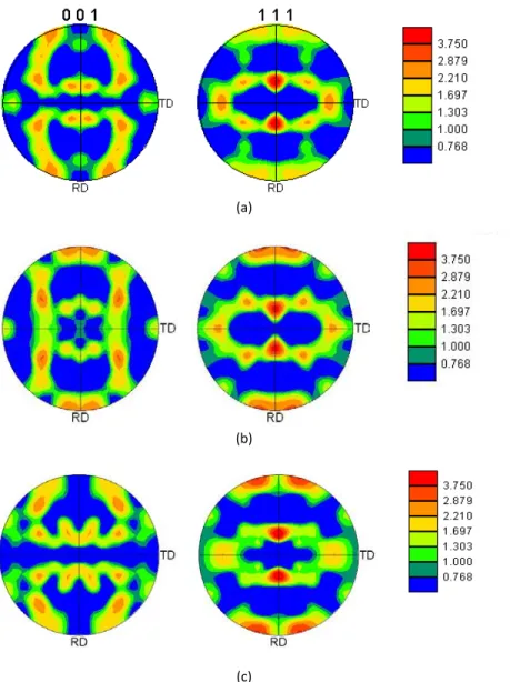
Figure 29: Predicted <0 0 1> and <1 1 1> pole figures for the (a) Top, (b) Middle and (c) Center sections at 60% thickness reduction ... 57

Figure 30: (a) Normal and (b) Shear strains in the rolling sample at different sections ... 59

Figure 31: Effective strain on rolled sample at different sections ... 59

Figure 32: Top section pole figures at 0%, 30% and 60% thickness reduction ... 60

Figure 33: (a) Neighbors of a single 3D element (b) Neighbor finding criterion ... 62

Figure 34: Grain algorithm (a) Initial (b) Final. Numbers inside the circles represent the Euler angles ... 63

Figure 35: Grains at (a) 0% thickness reduction and (b) 60% thickness reduction with random colors .... 64

Figure 36: Number of grains and grain size in the rolled sample using different misorientation angles ... 65

Figure 37: Rate of change of grains with respect to thickness reduction at different misorientations ... 66

Figure 38: Grain distribution across the sheet thickness in the pre-rolled (red) and rolled (blue) sample. Trend lines are added for ease of comparison ... 67

Figure 39: ODF plots for (a) small and (b) large grains at 60% thickness reduction ... 68

Figure 40: Combined undeformed ODF plot for small and large grains ... 69

Figure 41:ODF plots for (a) top section (b) center section at 0% thickness reduction ... 70

Figure 42:ODF plots at 60% thickness reduction for (a) small grains in the top section (b) small grains in the center section (c) large grains in the top section (d) large grains in the center section ... 71

Figure 43: Volume fraction data in the rolling sample at different thickness reductions ... 72

Figure 44: Normalized grain volume evolution in the rolling sample ... 72

Figure 45: Misorientation distribution of element neighbors in the rolled sample at 0%, 20%, 40% and 60% thickness reductions ... 73

Figure 46: (a) Normal strain and (b) Shear strain on top section (R stands for rolling and P stands for plane strain compression)... 75

Figure 47: Rolling <1 1 1> pole figures, plane strain compression <1 1 1> pole figures and difference pole figures at the top section at (a-c) 0%, (d-f) 30% and (g-i) 60% thickness reduction respectively . 76 Figure 48: Volume fractions of various texture components under Rolling (R stands for rolling, P stands for plane strain compression and T stands for Top section)... 77

Figure 49: Volume fraction comparisons of (a) Cube, (b) Copper, (c) S, (d) Brass and (e) Goss at top and center section (R stands for rolling, P stands for plane strain compression, T and C represent the top and center sections of the sample) ... 78

(13)

xiii

Figure 50: Plots of α and β fibers in Euler space [19] ... 79 Figure 51: ODF intensity comparisons of (a) γ-fiber and (b) at β-fiber top section between rolling and

plane strain compression (R stands for rolling and P stands for plane strain compression) ... 80 Figure 52: Experimental IPF map for AA 6063 ... 83 Figure 53: (a) Experimental and (b) Generated <111> pole figure for AA 6063 ... 83 Figure 54: Initial (a) Experimental and (b) Simulated AA 6063 texture shown as ODF plot (ϕ2-sections) . 84 Figure 55: Geometry and loading conditions applied ... 84 Figure 56: Calibrated AA 6063 data for h0, hs and τs ... 85 Figure 57: Calibrated surface for τ0 ... 86 Figure 58: Experimental and simulated AA 6063 uniaxial compression stress-strain curves at 0.01 s-1_{.... 87}

Figure 59: Experimental and simulated AA 6063 uniaxial compression stress-strain curves at 0.1 s-1_{... 87}

Figure 60: Experimental and simulated AA 6063 uniaxial compression stress-strain curves at 1 s-1_{... 88}

Figure 61: Experimental and simulated AA 6063 uniaxial compression stress-strain curves at 10 s-1_{... 88}

Figure 62: Experimental and simulated uniaxial compression stress-strain results for AA 6063 at 5000_{C 89}

Figure 63: Experimental deformed AA 6063 ODF plots (ϕ2-sections) at (a) 5000_{C 1 s}-1_{(b) 400}0_{C 0.01 s}-1

and (c) 4000_{C 1 s}-1_{... 91}

Figure 64: (a) Experimental and (b) Simulated AA 6063 ODF plots (ϕ2-sections) at 4000_{C 0.01 s}-1_{... 92}

Figure 65: Simulated deformed AA 6063 ODF plots (ϕ2-sections) at (a) 5000_{C 1 s}-1_{(b) 400}0_{C 0.01 s}-1_and

(c) 4000_{C 1 s}-1_{... 93} Figure 66: (a) Initial micrograph (black line represents 50 μm) (b) Deformed micrograph at 4000_{C 0.01 s}-1

(c) Deformed micrograph at 6000_{C 0.01 s}-1_{(d) Deformed micrograph at 400}0_{C 0.1 s}-1_{... 95}

(14)

xiv

List of Tables

Table 1: Typical texture components in FCC metals [84] ... 23

Table 2: Texture components by volume fraction in the initial sample ... 55

Table 3: Texture components by volume fraction in the deformed sample at 0 and 60% thickness reduction in the Top, Middle (Mid) and Center (Cen) sections ... 58

Table 4: Top section volume fraction difference at 30% and 60% thickness reduction for rolling and plane strain compression ... 77

Table 5: AA 6063 chemical composition (wt%)... 83

Table 6: Calibrated elastic values for AA 6063 ... 86

Table 7: Calibrated values for h0, hsand τs (AA 6063) ... 86

(15)

xv

Nomenclature

𝐹𝐹 Deformation gradient

𝜏𝜏𝛼𝛼 Resolved shear stress on slip system (𝛼𝛼)

𝛾𝛾̇(𝛼𝛼) Slip rates on slip system (𝛼𝛼) 𝑔𝑔(𝛼𝛼) Slip system (𝛼𝛼) hardness ℎ(𝛽𝛽) Single slip hardening ∅1,∅,∅2 Bunge Euler angles

𝑞𝑞0,𝑞𝑞1,𝑞𝑞2,𝑞𝑞3 Quaternion set

𝑏𝑏 Magnitude of burgers vector

𝑡𝑡 Time 𝜇𝜇 Shear modulus 𝜌𝜌 Dislocation density 𝜀𝜀̇ Strain-rate 𝑘𝑘 Boltzmann constant 𝜔𝜔𝑠𝑠𝑠𝑠𝑠𝑠𝑠𝑠𝑠𝑠ℎ Switching parameter

𝜉𝜉 Random number between 0 and 1

CPFEM Crystal plasticity finite element model

CPEFG Crystal Plasticity Element Free Galerkin Model

CA Cellular automata

JMAK Johnson Mehl Avrami Kolmogorov

SRX Static recrystallization

PSC Plane strain compression

gCode Grain Analysis Code

FE/FEA Finite element analysis

AAxxxx Aluminum alloy xxxx

FCC Face centered cubic

XFEM Extended finite element method

(16)

1

Chapter 1 Introduction

Aluminum alloys are increasingly being used in automotive applications due to their light weight, strength, formability and resistance to corrosion [1, 2]. Use of aluminum results in lighter cars with higher fuel efficiency while still meeting all the safety standards. As fuel costs rise, aluminum alloys provide the same or better cost-to-benefit ratio than steels and therefore are an ideal candidate for automotive industry. Automotive industry has been using aluminum alloys namely; AA 5754, AA 5182, AA 5083 from the early 1980’s for various automotive parts. The average net increase in rolled, extruded and die cast parts in automotive industry was around 20 Kg between 2012 and 2015 with the most increase in sheet and extrusions [3]. However, in recent years, many automotive manufacturers have substantially increased the aluminum content in their vehicles. For example, Fiat 500 has around 252 lbs. of aluminum while SUV’s like Chevy Suburban use 410 lbs. of aluminum [3]. Automotive manufactures use aluminum for manufacturing of car bodies, enclosures, transmission and subframe components [4]. Recently, Ford has designed the 2015 Ford F-150 Truck with an all aluminum body resulting in over 700 lbs. of weight reduction in saved body weight over previous models. This weight reduction has also led to an improved fuel consumption [3]. Similarly, 2007 Cadillac CTS uses aluminum alloys in chassis applications as a hollow casting/extruded welded cradle [4]. Audi R8, Honda NSX and many other vehicle manufacturers have also used various aluminum alloys for chassis applications [5]. Not only chassis or body, some automotive manufacturers have also used aluminum in transmission components. For example, Ford Motor Company’s Lincoln Mark VIII uses aluminum alloys in transmission components and recently even transmission blocks are being manufactured with aluminum alloys [5]. From the examples presented above, it is clear that there is a massive use of aluminum alloys in automotive applications and is expected to more than double in the next 10 years [3].

Use of aluminum sheet and extrusions shows the highest growth for automotive applications [3]. Aluminum sheets are produced from aluminum billets and are used in body panels such as doors, hoods, etc. Similarly, aluminum extrusions are used in body closures and body structures such as chassis, cradle, etc. In addition, use of aluminum sheets in automotive bodies is expected to drive the increase in aluminum content in automotive vehicles by 2025 [3]. As use of aluminum sheets and

(17)

2

extrusions increases, designers need to consider various parameters during sheet forming and extrusion processes to optimize and increase the efficiency of these processes.

To date, experimentation is the most common design approach for material and process characterization [4]. However, as experimental methods consume time and resources, there is an ever increasing need of numerical models to characterize material behavior to save experimental costs [6]. Numerical models generally require high computation and storage and there is a direct relationship between the model complexity and computation resources. With the advent of ever faster and efficient computers, numerical models are more accurate and can simulate more detailed/complex models. For example, earlier crystal plasticity models could only model single crystal under basic loading conditions to save computational resources [7]. However, recent models are able to simulate complex loading conditions with a polycrystal model that accounts for the complete material through thickness [8].

Finite element phenomenological models are commonly used to simulate deformation problems. Phenomenological models simulate the material behavior by fitting the simulated material response to experimental results under different loading conditions. However, phenomenological models are unable to capture the microstructure evolution in the material. Therefore phenomenological models cannot capture texture effects such as earing [6]. In addition, it is well known that mechanical properties such as ductility, strength and surface finish are directly affected by the sheet microstructure [9] and cannot be captured using phenomenological models. Crystal plasticity models offer a viable solution as they capture the material physics on each crystal/grain and are able to predict the material stress-strain and texture evolution during deformation. Crystal plasticity theory is the study of plastic behavior in materials due to crystallographic slip that accounts for the anisotropic material behavior in the material [10].

Crystal plasticity models require the starting texture of the material and therefore it is important to use the correct starting textures in crystal plasticity models. Experimental methods used to capture the texture and grain size information often do not match the model size in the simulation. Therefore, it is necessary to have a tool that creates synthetic textures that statistically match the bulk experimental texture. In addition, it should be possible to tailor these synthetic textures to any model size [11]. These synthetic textures, also known as synthetic microstructures, can then be used as inputs to crystal plasticity models.

(18)

3

Typical material testing processes such as tensile, compressive, etc. involve small strains. These have been simulated and validated for various materials using conventional phenomenological [12, 13] and crystal plasticity models [14, 15]. However, sheet forming (usually performed by rolling) and extrusions involve huge strains in the material and fall in the category known as large strain problems. As rolling and extrusion are large strain problems, conventional finite element methods are unable to simulate them. This is due to the mesh distortion and local inaccuracies in finite element methods at high strains. In order for automotive designers to simulate large strain problems, it is important to have a framework that is able to simulate large strain problems. In addition, large strain problems also involve huge microstructural changes. Therefore it is important to simulate the texture evolution (crystal plasticity) during these processes.

Currently, literature presents several methods to simulate crystal plasticity based large strain problems such as rolling. Taylor type models are the most commonly used models in literature as they provide fast and efficient solutions to crystal plasticity problems [16, 17]. However, Taylor type models assume constant strain in each grain which can result in erroneous stress states in the material. Taylor type and other crystal plasticity models have been used to simulate rolling by assuming a plane strain compression condition (e.g. [18, 19]). Yet, they are unable to capture the through thickness of the sheet. Experimental results show that it is important to capture the through thickness of the sheet as the material undergoes inhomogeneous deformation due to different strain paths experienced at different material thickness in the rolled sheet [20, 21]. For example, Figure 1 shows that the volume fraction of Rolling Texture and Shear Texture increases down the sheet thickness. In addition experimental results from literature also show a change in the grain size across the thickness of the sheet [21]. Therefore it is important to capture the through thickness of the sheet with the correct loading conditions when simulating cold rolling.

(19)

4

Figure 1: Volume fraction of different texture components at various sheet thickness depths [21]

It is important to consider the complete through thickness of the sheet with the correct loading conditions to capture the material stress-strain and texture evolution during cold rolling. FEM are the most common tool used to simulate large strain problems. However, as conventional FE cannot capture the texture evolution, crystal plasticity theory has been implemented to classical Finite Element Methods (CPFEM) to capture the texture evolution. In addition, literature presents various applications of CPFEM models (e.g. [10]). However, finite element formulations are prone to errors at higher strains due to high element distortion. Re-meshing is the most common technique used to overcome this problem. Re-meshing has been used successfully to model large strain problems such as extrusion. However, CPFEM models cannot work with re-meshing as each new element needs to be assigned a new orientation. Element Free Galerkin (EFG) methods provide a viable solution to this problem [22]. EFG problems have also been used to model crack and fracture problems [23]. EFG methods are meshless methods. They have also been shown to be more accurate than finite element methods as they do not accumulate numerical errors caused by distorted elements in FE models (Figure 2). Therefore an EFG based crystal plasticity framework needs to be developed to accurately model large strain problems such as rolling.

(20)

5

Figure 2: Experimental (Exact), simulated Finite Element Methods (FEM) and Element Free Galerkin (EFG) results for hole in an infinite plate [23]

Like rolling, hot compression is also a large strain problem and induces huge strains in the material. Hot compression is used as a stepping stone to understand the extrusion processes as they are both performed at high temperatures. In addition, like extrusion, hot compression can also be performed at different strain-rates. As hot extrusion can be carried out at various temperatures and strain-rates, it is important to include those effects in the crystal plasticity model. Currently, literature lacks modelling approaches to characterize and model the flow behavior and texture evolution of aluminum alloys (such as AA 6xxx) under different temperatures and strain-rates. Therefore there is a need to develop a strain-rate and temperature dependent crystal plasticity model to simulate large strain processes such as hot compression.

Experimental results show that aluminum alloys (e.g. AA 6xxx) undergo static recrystallization (Figure 3) at high temperatures [24, 25]. Static recrystallization involves identifying potential nuclei and their growth. Material that undergoes SRX results in a different material texture and grain size than the one without SRX. Therefore, material with and without SRX result in different mechanical properties. Therefore, it is very important to consider the effects of SRX after hot deformation to predict the correct texture and grain size. Hence, a through process model (crystal plasticity and SRX) is needed to model the material behavior, texture and grain size during hot compression.

(21)

6

(a) (b)

Figure 3: (a) Optical micrograph and (b) TEM images for AA 6063 under high temperatures [25]

The main objective of this research is to model and analyze the stress-strain and microstructure changes during large strain problems namely; cold rolling and hot compression. A rate-dependent crystal plasticity based Element Free Galerkin (CPEFG) constitutive model was developed to model cold rolling in AA 5754. CP model was implemented in commercial software LS-DYNA as a user defined EFG material model (UMAT) to simulate the 3D microscopic response of AA 5754 under cold rolling. Simulated model captured the complete through thickness of the sheet. Results from CPEFG simulations were compared to experimental data and showed good agreement. A more detailed description of the CPEFG model, validation and implementation to cold rolling is given in Section 6.1. Crystal plasticity simulations predict the overall texture and grain size in the material. However, this information can be used to calculate other grain metrics such as grain size, subgrain formation, texture preference, etc. Accurate grain size predictions during and after rolling are important as they relate to the material properties such as yield strength through the Hall-Petch effect [26]. It is well known that under certain deformations such as shear [27], FCC materials prefer certain texture components and predicting the development of these texture components is essential to any model. To study the evolution of texture components and other grain metrics, new tools need to be developed. Therefore, in this research, grain size and preferred textures for small and large grains near the top and center of the sheet were studied using an in-house grain analysis framework (gCode). In-house gCode is based on a neighbor misorientation path finding algorithm [28] to study the subgrain formation. More details about the gCode are discussed in Section 6.1.5.

(22)

7

In the second part of this work, hot compression was modelled using an in-house crystal plasticity Taylor model. A modified hardening CP model was used to model hot compression in AA 6063 under different temperatures and strain-rates. As hot compression involves SRX, a probabilistic integration point based SRX model was developed to model SRX at various temperatures and strain-rates. Simulated stress-strain, texture and grain size results were compared to experimental results. The Electron Back Scatter Diffraction (EBSD) on the initial AA 6063 was performed by Waqas Muhammad (a fellow student) while the hot compression Gleeble experiments were performed by Daniel Ohoh (PhD student with Prof. Marry Wells at University of Waterloo). More details about the modified hardening crystal plasticity model and SRX are discussed in Section 6.3.

In summary, the main objective of this work is to model and analyze the microstructure changes during large strain processes in FCC polycrystals. To accomplish this objective, this thesis is arranged as follows: Chapter 2 discusses the crystal plasticity theory, numerical models and microstructures used in numerical models. Chapter 3 discusses recrystallization and various approaches to simulate recrystallization. Chapter 4 discuss the overall scope and objectives of this work. Chapter 5 discusses the crystal plasticity and static recrystallization frameworks used in this work. Chapter 6 discusses the main results and presents the simulated cold rolling results from CPEFG simulations. Next, gCode is used to analyze various through thickness grain metrics under cold rolling. Chapter 6 also discusses the stress-strain, texture and grain size evolution during hot compression and validates the simulated results with experimental data. Lastly, Chapter 7 looks at limitations of current work and future work to improve the various modelling approaches presented in this work.

(23)

8

Chapter 2 Numerical Modelling

Computer simulations provide a huge advantage over conventional experimental approaches to model material behavior such as cost, time, etc. Therefore there is a huge push to accurately model the material behavior under different loading conditions using different types of numerical techniques. Conventional phenomenological models [29, 30, 12, 31–33] provide material stress-strain response and are adequate for most applications but do not account for material texture evolution. Crystal plasticity approaches solve this problem by accounting for material texture and are discussed below.

There are a number of ways to model large strain crystal plasticity problems. Taylor and Sachs approaches have been used with great success in literature [16, 17, 14] and can account for material texture evolution on an average sense. Other approaches such as Crystal Plasticity Finite Element Methods (CPFEM) are also used to model large strain problems. CPFEM methods can account for the complete material microstructure. In addition, CPFEM approaches provide full-field solutions and are discussed in more detail in Section 2.2. However, finite element methods do not allow for severe deformations due to mesh restrictions. In addition, high mesh distortion during deformation affects the final results in FEA simulations. FEA has been modified to Extended Finite Element Method (XFEM) which allows the study of failure and fracture in materials. New approaches such as meshless methods (EFG) provide the flexibility of severe deformations without mesh dependence. All the methods mentioned above solve a finite element ordinary differential equation with minor changes to its implementation in the final framework. These methods are briefly summarized below.

2.1 Crystal Plasticity Theory

2.1.1 Introduction

Metals are crystalline solids consisting of atoms arranged in different patterns. These patterns are repeated in all directions. This atomic arrangement can be described using unit cells as shown in Figure 4[34]. Figure 4shows the unit cells for typical metallic unit cells namely; face-centered cubic (FCC), body-centered cubic (BCC) and hexagonal close-packed (HCP). Some of the metals that have FCC crystal lattice structure are aluminum, 𝛾𝛾-iron, copper, brass, nickel etc. 𝛽𝛽-iron, potassium and molybdenum belong to BCC while magnesium, titanium and zirconium belong to HCP lattice. In the present research proposal, focus is on FCC metals only.

(24)

9

Figure 4: Unit cells of BCC (Body-centered cubic), FCC (Face-centered cubic) and HCP (Hexagonal closed packed) [34]

Real crystals contain imperfections in their lattice. These lattice imperfections could be as a point, line or interfacial defects. Point defects include interstitial atoms, vacancies and impurity atoms. Most important line imperfections are known as dislocations. Dislocations can be described as areas where atoms are out of place in the crystal lattice. This results in namely two type of dislocations; edge and screw. Edge dislocation centers on a line that is defined along an extra half-plane of atoms. Some atoms above this line are squeezed together and some are pulled apart. Screw dislocation is thought to be formed due to shear stress where one part of the crystal lattice moves relative to the other by one atomic distance. Interfacial defects include boundaries which separate crystallographic regions with different crystallographic orientations and include grain boundaries, twins, stacking faults and phase boundaries [35].

Plastic deformation occurs mostly due to movement of dislocations (line-defects). Concept of dislocations was proposed by Taylor [36] as the shearing of rows of atoms in a crystal propagating throughout the crystal with change in temperature and strain. Any applied stress can be transformed into shear stress on the glide plane of any dislocation. This is known as the resolved shear stress and is the cause of dislocation movement. FCC metals at room temperature have several plastic deformation mechanisms namely; slip, twinning and grain boundary sliding. However, slip is the principal mechanism of deformation. Therefore, only this mechanism is considered in this research proposal.

Dislocations have preferred planes and directions within those planes where motion occurs. The planes are called slip planes and directions are called slip directions. The combination of these is called a slip system. Slip systems depend on the crystallographic structure of the metal. Due to different slip systems, crystallographic slip is anisotropic. A FCC unit cell is shown in Figure 5a. A [1 1 1] type plane

(25)

10

is shown in the unit cell. Slip occurs along the <1 1 0> directions within the [1 1 1] slip plane. The number of independent slip systems represents the different combinations where slip can occur. For FCC, there are four unique [1 1 1] planes and three <1 1 0> directions per plane resulting in 12 unique slip systems.

(a) (b)

Figure 5: (a) A [1 1 1] <1 1 0> Slip System in FCC unit cell (b) [1 1 1] Plane from (a) and three slip directions within the [1 1 1] plane (shown by arrows) [35]

Stress applied to a material can be resolved into shear stresses on slip planes and directions. On application of a stress, there is a most favorable slip system for a crystal. When the resolved shear stress reaches a critical value, this slip system undergoes slip. This shear stress is called the critical shear stress. This is known as the Schmid’s Law [37]. Schmid Law is used to serve as a yield criterion for a single crystal. Schmid’s Law states that extensive slip occurs when the resolved shear stress reaches a critical value. Therefore, a single crystal yields or deforms plastically, when the resolved shear stress reaches the critical resolved shear stress; i.e. when,

𝜏𝜏𝛼𝛼=𝑚𝑚𝛼𝛼,𝑠𝑠𝑖𝑖𝜎𝜎𝑠𝑠𝑖𝑖 =𝜏𝜏𝑦𝑦,𝛼𝛼(𝑖𝑖,𝑗𝑗= 1,2,3) (1)

where 𝜏𝜏𝛼𝛼is the resolved shear stress for a slip system (𝛼𝛼). 𝜎𝜎𝑠𝑠𝑖𝑖 is the stress acting on the crystal, 𝜏𝜏𝑦𝑦 is

the yield strength of 𝛼𝛼 slip system and 𝑚𝑚𝛼𝛼,𝑠𝑠𝑖𝑖 is defined as,

𝑚𝑚𝛼𝛼,𝑠𝑠𝑖𝑖 =𝑠𝑠𝛼𝛼,𝑠𝑠𝑏𝑏𝛼𝛼,𝑖𝑖 (2)

where 𝑠𝑠𝛼𝛼,𝑠𝑠 and 𝑏𝑏𝛼𝛼,𝑖𝑖 are the components of the slip vectors 𝑠𝑠𝛼𝛼and slip normal 𝑏𝑏𝛼𝛼 for slip system 𝛼𝛼

respectively. It should be noted that throughout this report, the usual convention of tensor summation is implied on 𝑖𝑖,𝑗𝑗 whereas 𝛼𝛼 refers to the slip system.

(26)

11

2.1.2 Single Crystal Deformation Models

Properties of polycrystals can be derived from single crystal properties. This section discusses the rate-dependent and inrate-dependent crystal plasticity formulations. Both formulations account for plastic deformation using crystallographic slip but have certain advantages.

2.1.2.1 Rate Independent Models

Schmidt law yields simple flow rules for shear rates (𝛾𝛾̇𝛼𝛼) for a slip system according to the rate

independent crystal plasticity theory. Rules state that;

a. 𝛾𝛾̇𝛼𝛼 = 0 when current value of yield stress (𝜏𝜏𝑦𝑦,𝛼𝛼) is greater than the resolved shear stress (𝜏𝜏𝑦𝑦).

b. 𝛾𝛾̇𝛼𝛼 = 0 when 𝜏𝜏𝑦𝑦,𝛼𝛼 =𝜏𝜏𝑦𝑦 and rate of resolved shear stress is less than slip system hardening

matrix (ℎ𝛼𝛼𝛽𝛽) times the increment of rate of shear (𝛾𝛾̇𝛽𝛽) and

c. 𝛾𝛾̇𝛼𝛼 = 0 when 𝜏𝜏𝑦𝑦,𝛼𝛼=𝜏𝜏𝑦𝑦 and rate of resolved shear stress is equal to the slip system hardening

matrix (ℎ𝛼𝛼𝛽𝛽) times the increment of rate of shear (𝛾𝛾̇𝛽𝛽)

These rules characterize inactive, active and potentially active systems. Crystal plasticity theory by Taylor [38] states that only five independent slip systems out of 12 slip systems (for FCC) are required to completely prescribe any arbitrary strain. To select these active slip systems, it was suggested to use the combination of slip systems that yield the minimum shear rates. This was suggested based on single crystal experimental results [38]. This theory was also explained by the principle of maximum work [39]. It was shown by Chin and Mammel [40] that the theory of maximum work and minimum shear works out to be the same [41].

2.1.2.2 Rate Dependent Models

Yield surface of a rate-independent formulation is a polyhedron which has sharp corners. Sharp corners results in lack of uniqueness in the choice of actively yielding slip systems due to lack of uniqueness of the strain-rate vector perpendicular to the edges of the polyhedron. Another problem is that if the stress is on the corner of this yield surface, six or eight slip systems could be activated simultaneously corresponding to non-unique slips.

In order to resolve the ambiguities mentioned above, rate sensitivity was introduced into Taylor type models [42]. This method did not have explicit yielding of slip systems but assumed that all slip systems slip at a rate based on the current value of resolved shear stress. Due to the unique relation

(27)

12

between slip rates and stress states, the slip rate on each slip system could be determined uniquely. This solved the problem of non-uniqueness in stress states of rate independent solutions.

2.1.3 Polycrystal Models/Mean Field Homogenized Approach

In order for crystal plasticity models to predict real material response, they have to capture polycrystalline response. However, a polycrystal model must be able to offer more than a phenomenological model. It should be able to capture and explain phenomenon that phenomenological models are unable to e.g. texture, microstructure evolution, grain morphology. Accurate prediction of texture evolution is very important as many forming operations (e.g. stamping) are texture dependent. In general single crystal models which already have the required parameters such as slip, twinning, etc. included in them can be adapted to polycrystal models. Polycrystal models discussed below are mean field models and provide average response of the crystal. They are known as mean field or homogenized models as they capture the polycrystalline response in the average sense.

2.1.3.1 Sachs Model

Early polycrystalline models made some continuity assumptions across grains. Sach’s model [43] assumes that all grains in a model are subjected to the same stress state. Sach’s model also assumes that only one slip system is active at any moment in time in each grain. This model was later modified so that each grain was assumed to be subjected to the same strain [44]. The assumption that each grain experiences the same stress ignores the strain continuity across grain boundaries [39]. In addition, some numerical inconsistencies were also observed by Asaro and Needleman [42].

2.1.3.2 Taylor Model

Taylor’s model assumes the same strain per grain but requires 5 slips systems to be active at once (for FCC). Selection of five slip systems to minimize slip results in checking all possible combinations (384 for FCC structure). Strain is found by applying a volume average across all grains and hence is known as a full constraint model. The Taylor model also accommodates for the strain continuity across grain boundaries.

Taylor model was based on experimental observations of a cross-section of a drawn wire. Taylor observed that all grains were elongated in the direction of extension. This lead to the conclusion that each grain experienced the same strain. In addition, each grain deforms in exactly the same way inside a polycrystal and satisfies:

(28)

13 𝜎𝜎𝑔𝑔 𝜏𝜏 = 𝑑𝑑𝛾𝛾 𝑑𝑑𝜀𝜀 =𝑀𝑀 (3)

where 𝜎𝜎𝑔𝑔 is the axial stress in a grain, 𝜏𝜏 is the shear strength, 𝑑𝑑𝛾𝛾 and 𝑑𝑑𝜀𝜀 are the increments in

shear-strain and aggregate shear-strain and 𝑀𝑀 is the orientation factor that depends on the lattice orientation. However this implies abrupt changes in stress between neighboring grains based on their orientations. This can cause numerical instabilities as reported by Bishop and Hill [45, 46].

The simplicity of the Taylor approach has been applied in combination with other numerical methods such as Finite Element Methods. Experimental works have proven that the equal strain assumption used in the Taylor model is not true. However, the Taylor model has been used in simulating various problems with accurate results particularly in the prediction of forming limit diagrams [16, 17, 14]. A modification of the Taylor model, known as the relaxed constraints model has also been implemented [47]. By relaxing the compatibility constraints, this type of model has been used to predict texture evolution in FCC metals. Relaxed constrains model has also shown improvements over the Taylor model under simple shear [48].

2.1.3.3 Viscoplastic Self Consistent Model (VPSC)

A consistent polycrystal model was proposed by Kroner [49] and Hill [50]. This was a self-consistent model, based on Eshelby’s formulation [51], that treated the deformation of each grain as the solution for an elastic elliptical inclusion within a homogenous matrix average across all the grains. Lebensohn et al. [52] extended this model to predict the stress-strain as well as texture evolution. This model was later revised to include plasticity by introducing the viscoplastic self-consistent (VPSC) scheme[53]. Self-consistent models find the local strains by averaging the response between different grains. VPSC model uses the Eshelby’s inclusion model [51]and links the average strain-rate (𝜀𝜀̅(𝑟𝑟)_{) to} the average eigen strain-rate (𝜀𝜀̅∗(𝑟𝑟)_{) using the Eshelby tensor (}_𝑆𝑆_{). The model assumes each grain as an} elliptical inclusion in a viscoplastic medium where the material response for the grain and medium is given by: 𝜀𝜀(𝑟𝑟)₌_𝛾𝛾 0� 𝑚𝑚𝑘𝑘(𝑟𝑟) 𝑘𝑘 �𝑚𝑚𝑘𝑘(𝑟𝑟):𝜎𝜎(𝑟𝑟) 𝜏𝜏₀𝑘𝑘(𝑟𝑟) � 𝑛𝑛 ₍₄₎

where 𝜀𝜀(𝑟𝑟)_{is the strain on each grain (}_𝑟𝑟_),_𝜏𝜏

0𝑘𝑘(𝑟𝑟) is the resolved shear stress on each slip system (𝑘𝑘), 𝛾𝛾0

(29)

14

The VPSC model has been used extensively for FCC, BCC and HCP materials (such as [54, 55]). VPSC model has been shown to accurately predict the stress-strain response and texture evolution under complex strain paths, such as rolling [56].

2.2 Full-Field Models

Mean field models mentioned in the previous section provide the average behavior of the material but are unable to capture important material phenomenon such as intra-granular stresses, grain breakage, grain-to-grain interaction, etc. Full field models provide the ability to study these phenomenon in detail as they do not use any averaging scheme to find local strains and are discussed below.

2.2.1 Finite Element Analysis (FEA)

Finite Element Analysis has been used extensively to model deformation problems. Phenomenological models try to model the physics of deformation by incorporating various mathematical expressions to experimental results. Phenomenological models have been shown to predict material response under all types of loading conditions, strain-rates and temperatures (such as [12, 31, 57–59]). Unlike earlier models [60], recent phenomenological models can account for the material asymmetry and anisotropy [12, 31]. However, FE based models can also be implemented with crystal plasticity framework to account for the texture evolution. FE models provide the advantage of full-field approach which can accurately account for the texture evolution and intra-granular material behavior [8, 61–64]. As mentioned earlier, FE models can also be combined with other models e.g. Taylor model to provide full and relaxed constraints model. Basic FE models try to find the solution to the momentum equation

𝜎𝜎𝑠𝑠𝑖𝑖+𝜌𝜌𝑓𝑓𝑠𝑠 =𝜌𝜌𝑥𝑥̈𝑠𝑠 (5)

Satisfying the traction and displacement boundary conditions

𝜎𝜎𝑠𝑠𝑖𝑖𝑛𝑛𝑠𝑠=𝑡𝑡𝑠𝑠(𝑡𝑡) (6)

𝑥𝑥𝑠𝑠(𝑋𝑋𝑎𝑎,𝑡𝑡) =𝐷𝐷𝑠𝑠(𝑡𝑡)

(30)

15

where 𝜎𝜎 is the Cauchy stress, 𝜌𝜌 is the density of the material, 𝑓𝑓 is the body force,𝑡𝑡 is the traction, 𝑥𝑥̈ is the acceleration of the body and 𝜎𝜎𝑠𝑠𝑖𝑖+ and 𝜎𝜎𝑠𝑠𝑖𝑖−are the stresses on boundary. This leads to the weak

form of the equilibrium equation: 𝛿𝛿𝛿𝛿=� 𝜌𝜌𝑥𝑥̈𝑠𝑠𝛿𝛿𝑥𝑥𝑠𝑠𝑑𝑑𝑑𝑑

𝑣𝑣 +� 𝜎𝜎𝑣𝑣 𝑠𝑠𝑖𝑖𝛿𝛿𝜀𝜀𝑠𝑠𝑑𝑑𝑑𝑑 −� 𝑓𝑓𝑣𝑣 𝑠𝑠𝛿𝛿𝑥𝑥𝑠𝑠𝑑𝑑𝑑𝑑 −� 𝑡𝑡𝑏𝑏 𝑠𝑠𝛿𝛿𝑥𝑥𝑠𝑠𝑑𝑑𝑠𝑠

= 0

(7)

This equation complies with the principle of virtual work that states that a body in equilibrium and subjected to displacements will have the virtual work of external forces on the body equal to the virtual strain energy of the internal stresses [65].

Next, introduce the mesh in finite elements and re-write Equation 7 in terms of shape functions (𝑁𝑁𝑠𝑠)

� �� 𝜌𝜌𝑢𝑢̈𝑠𝑠𝑁𝑁𝑠𝑠𝑚𝑚𝑑𝑑𝑑𝑑 𝑣𝑣𝑚𝑚 +� 𝐵𝐵𝑠𝑠𝑖𝑖𝑚𝑚𝑠𝑠𝐷𝐷𝑠𝑠𝑖𝑖𝑚𝑚𝐵𝐵𝑠𝑠𝑖𝑖𝑚𝑚𝑁𝑁𝑠𝑠𝑚𝑚𝑢𝑢𝑠𝑠𝑚𝑚𝑑𝑑𝑑𝑑 − 𝑣𝑣𝑚𝑚 � 𝑓𝑓𝑠𝑠𝑚𝑚𝑁𝑁𝑠𝑠𝑚𝑚𝑑𝑑𝑑𝑑 − 𝑣𝑣𝑚𝑚 � 𝑡𝑡𝑠𝑠𝑚𝑚𝑁𝑁𝑠𝑠𝑚𝑚𝑑𝑑𝑠𝑠 𝑏𝑏 � 𝑛𝑛 𝑚𝑚=1 = 0 (8)

where strain (𝜀𝜀) and stress (𝜎𝜎) is written in terms of nodal displacements and displacements are approximated by nodal displacements (𝑢𝑢) using:

𝜀𝜀=𝐵𝐵𝑥𝑥, 𝑥𝑥=𝑁𝑁𝑢𝑢,𝜎𝜎=𝐷𝐷𝜀𝜀 (9)

We can re-write this equation in matrix form, � �� 𝜌𝜌𝑁𝑁𝑠𝑠_{𝑁𝑁𝑢𝑢̈𝑑𝑑𝑑𝑑} 𝑣𝑣𝑚𝑚 +� 𝐵𝐵𝑠𝑠_{𝐷𝐷𝐵𝐵𝑑𝑑𝑑𝑑𝑢𝑢 −} 𝑣𝑣𝑚𝑚 � 𝑁𝑁𝑠𝑠_{𝑓𝑓𝑑𝑑𝑑𝑑 −} 𝑣𝑣𝑚𝑚 � 𝑁𝑁𝑠𝑠_{𝑡𝑡𝑑𝑑𝑠𝑠} 𝑏𝑏 � 𝑛𝑛 𝑚𝑚=1 = 0 (10)

These expressions can be expressed as

[𝑀𝑀][𝑢𝑢̈] + [𝐾𝐾][𝑢𝑢] = [𝐹𝐹] (11)

(31)

16

2.2.2 Extended Finite Element Method (XFEM)

Extended Finite Element Method (XFEM) was developed to predict crack initiation and propagation [66, 67]. The key idea is that the displacement equation incorporates the crack discontinuity as an additional term in the finite element formulation [68]. Displacement is given as [69]:

𝑢𝑢ℎ₍_𝑋𝑋_,_𝑡𝑡_{) =}_{� 𝑁𝑁}

𝐼𝐼(𝑋𝑋){𝑢𝑢𝐼𝐼(𝑡𝑡) + 𝐻𝐻�𝑓𝑓(𝑋𝑋)�𝐻𝐻�𝑔𝑔(𝑋𝑋,𝑡𝑡)�𝑞𝑞𝐼𝐼} (12)

where NI(x) is a shape function, and 𝑢𝑢_𝐼𝐼and 𝑞𝑞_𝐼𝐼 are the regular and enriched nodal values respectively.

𝐻𝐻�𝑓𝑓(𝑋𝑋)� is the Heaviside function which is active only when 𝑓𝑓(𝑋𝑋) is greater than zero. Functions f(x) and g(x) define the continuous crack geometry in the material shown in Figure 6.

Figure 6: Discontinuity representation in XFEM [69]

The main disadvantage of XFEM is the additional CPU time. In addition, XFEM simulations cannot predict crack speeds and multiple cracks unless the model is tuned with the experimental results [69]. XFEM simulations also require the user to input the discontinuity on the basis of some failure criterion to predict cracks.

As discussed, XFEM was developed for crack problems and does not provide the flexibility of incorporating severe deformations in its formulation. Severe deformation can be incorporated with XFEM by using adaptive meshing techniques. However, these techniques require huge computational times.

(32)

17

2.2.3 Element Free Galerkin (EFG)

EFG is a relatively new mesh-less numerical method [70]. Unlike classical FE simulations, EFG methods use only nodes and do not require elements. This makes it easier to mesh complex parts and geometries. Even though re-meshing allows FE models to simulate complex strain paths [71], nodal mesh in EFG simulation allows for simulating high deformation problems without re-meshing. EFG is based on the partition of unity method [72] and elements in EFG are called cells. In FE methods, cells are known as elements and are predefined by the user. However, in EFG, cells are calculated based on the problem definition and can be calculated based on a fixed or variable radius from the current point. This could result in different cells with different number of points. In addition, cells in EFG could also be squares, circles (2D) or cubes, spheres (3D). These cells can be static or evolve during simulations. A sample of circular cells in a given domain is shown in Figure 7.

Figure 7: EFG cells in a sample [73]

EFG employs moving least square (MLS) approximants to approximate the displacement functions. These approximations consist of a weight function, a polynomial basis and position based coefficients. A linear approximation of displacement (𝑢𝑢) can be written as:

𝑢𝑢ℎ₍_𝑥𝑥_{) =}_𝑎𝑎

0(𝑥𝑥) +𝑎𝑎1(𝑥𝑥)𝑥𝑥 (13)

(33)

18

The MLS approximation in the whole domain is given by [23]:

𝑢𝑢ℎ₍_𝑥𝑥_{) =}_{� 𝑝𝑝} 𝑠𝑠 𝑚𝑚 𝑠𝑠=1 (𝑥𝑥)𝑎𝑎𝑠𝑠(𝑥𝑥) =𝑝𝑝𝑇𝑇(𝑥𝑥)𝑎𝑎(𝑥𝑥) (14)

where 𝑝𝑝𝑠𝑠 are the components of the monomial basis function and 𝑎𝑎𝑠𝑠 are their coefficients. The

coefficients are found by minimizing a weighted discrete 𝐿𝐿2 norm and depends on the weight function

and the neighborhood of 𝑥𝑥. A linear basis in 3D is given as:

𝑝𝑝𝑇𝑇₍_𝑥𝑥_{) = [1,}_𝑥𝑥_,_𝑦𝑦_,_𝑧𝑧_] ₍₁₅₎

This stationarity of the 𝐿𝐿2 norm with respect to 𝑎𝑎(𝑥𝑥) to the following linear relation:

𝐴𝐴(𝑥𝑥)𝑎𝑎(𝑥𝑥) =𝐵𝐵(𝑥𝑥)𝑢𝑢 (16)

where 𝐴𝐴(𝑥𝑥) and 𝐵𝐵(𝑥𝑥) are defined in terms of the weight functions (𝑤𝑤) and monomial basis (𝑝𝑝). Weight function (𝑤𝑤) should be constructed to be positive and guarantee a unique solution to 𝑎𝑎(𝑥𝑥). Generally EFG weight functions are more complicated than finite element weight functions and are available as exponential, cubic and quartic-spline functions. A simple weight function (based on distance) can be written as:

𝑤𝑤(𝑥𝑥 − 𝑥𝑥𝑠𝑠) = ||𝑥𝑥 − 𝑥𝑥𝑠𝑠|| (17)

Substituting 14 into 16 results in

𝑢𝑢ℎ 𝑠𝑠(𝑥𝑥) =� 𝑁𝑁𝑠𝑠(𝑥𝑥) 𝑚𝑚 𝑠𝑠=1 𝑢𝑢𝑠𝑠 (18)

where 𝑁𝑁𝑠𝑠(𝑥𝑥) =𝑝𝑝𝑇𝑇𝐴𝐴−1𝐵𝐵𝑠𝑠 is the shape function to approximate the nodal displacement (𝑢𝑢𝑠𝑠).

The rest of the EFG problem simplifies to a set of integrals, similar to any other finite element problem. Unlike finite element problems, that loop on each element, EFG problems loop on each quadrature point (𝑚𝑚). The main disadvantage of the EFG method is that they require very large CPU time and EFG simulations can take 2-3 times longer than “classical” FE models for the same problem. This is due to the relatively complicated weight functions and shape function approximations used in EFG.

(34)

19

2.2.4 Fast Fourier Transform Method (FFT)

As discussed above, Finite Element Methods have been used extensively to account for different types of material problems. However, due to the large number of degrees of freedom required by FE methods, there is an inherent size limitation based on the computational resources. FFT methods provide an effective alternate solution as they can account for fine-scale microstructural information that is hard to achieve with FE methods. However, FFT methods assume periodicity and require periodic conditions across the length of the sample. Hence FFT methods are not as versatile as FE methods.

Moulinec and Suquet [74] initially proposed a FFT based method for composites which was later used by Lebensohn [75] to model viscoplastic polycrystals and then elasto-viscoplastic polycrystals [76]. The basic FFT framework works on a 3D point grid with a fixed amount of Fourier points in each direction and a periodic boundary across the RVE where the total strain and stress are given by:

𝜖𝜖(𝑥𝑥) =𝑒𝑒̃(𝑥𝑥) +𝐸𝐸 𝜎𝜎(𝑥𝑥) =𝐶𝐶0:𝜖𝜖(𝑥𝑥)

(19)

where e�(𝑥𝑥) is the strain fluctuation in the crystal, ϵ(x) is the local strain field, E is the average strain in the material, 𝜎𝜎(𝑥𝑥) is the stress field and 𝐶𝐶0 is the initial local elastic stiffness matrix.

The local fluctuation of the displacement field is calculated using the Green function as: 𝑒𝑒̃𝑘𝑘(𝑥𝑥) =� 𝐺𝐺𝑘𝑘𝑠𝑠(𝑥𝑥 − 𝑥𝑥′)𝜏𝜏𝑠𝑠𝑖𝑖,𝑖𝑖(𝑥𝑥′)𝑑𝑑𝑥𝑥′

𝑅𝑅3

(20)

where 𝐺𝐺(𝑥𝑥 − 𝑥𝑥′₎_{is the Green function and}_𝜏𝜏_{is the shear stress. Using Equation 19 and converting}

this expression into Fourier space results in:

𝑒𝑒̃𝑠𝑠𝑖𝑖(𝑥𝑥) =𝛤𝛤�𝑠𝑠𝑖𝑖𝑘𝑘𝑖𝑖 ∗ 𝜏𝜏̂𝑘𝑘𝑖𝑖 (21)

where Γ� can be calculated as:

𝛤𝛤�𝑠𝑠𝑖𝑖𝑘𝑘𝑖𝑖 =−1_{2 (}𝜉𝜉𝑠𝑠𝜉𝜉𝑖𝑖𝐴𝐴′𝑠𝑠𝑘𝑘−1+𝜉𝜉𝑠𝑠𝜉𝜉𝑖𝑖𝐴𝐴′−1𝑠𝑠𝑘𝑘 )

(22)

(35)

20

2.3 Orientation Space

Orientations are used to completely describe a relation between two coordinate frames. Similarly, material texture is defined as a set of orientations corresponding to all the crystals in the material. Orientations are represented usually in Euler space as Bunge angles (𝜑𝜑1,∅,𝜑𝜑2) to describe the crystal

orientation with respect to the global space [77]. This space is finite and is used to describe any texture component by a single point where texture is defined as a non-uniform distribution of crystallographic orientations in a polycrystalline aggregate [78]. Bunge angles describe this point as an anticlockwise rotation about z-x-z axis. As shown in Figure 8, this can be described as a rotation about [0 0 1] (ND - Red), [1 0 0] (Green) and [0 0 1] (Blue) crystal direction.

Figure 8: Rotation in Euler space on crystal axis [79]

Orientations in 3D space can also be represented using quaternion’s (𝑞𝑞0,𝑞𝑞1,𝑞𝑞2,𝑞𝑞3) such that

∑ 𝑞𝑞𝑠𝑠 = 1. Quaternion space is defined by a scalar (𝑞𝑞0) and a vector. Quaternions are used due to the

ease of normal mathematical operations when using multiple quaternion’s [80]. For example, addition of two quaternions (𝑎𝑎,𝑏𝑏) is given as:

𝑎𝑎+𝑏𝑏= (𝑎𝑎0+𝑏𝑏0), (𝑎𝑎1+𝑏𝑏1), (𝑎𝑎2+𝑏𝑏2), (𝑎𝑎3+𝑏𝑏3) (23)

Crystal plasticity framework implemented in this work use Euler space while all the calculations to calculate misorientation are performed in quaternion space. Therefore it was necessary to define functions that could be used to switch between these spaces while maintaining the FCC symmetry conditions.

(36)

21

A rotation angle/axis pair (𝑤𝑤,𝑛𝑛) can also be used to describe a quaternion [81] and the relationship between a quaternion and Euler angles can be written as:

±𝑞𝑞= ±�𝑐𝑐𝑐𝑐𝑠𝑠 �𝑤𝑤₂�,𝑠𝑠𝑖𝑖𝑛𝑛 �𝑤𝑤₂� 𝑛𝑛1,𝑠𝑠𝑖𝑖𝑛𝑛 �𝑤𝑤₂� 𝑛𝑛2,𝑠𝑠𝑖𝑖𝑛𝑛 �𝑤𝑤₂� 𝑛𝑛3� = ±�𝑐𝑐𝑐𝑐𝑠𝑠 �𝛽𝛽₂� 𝑐𝑐𝑐𝑐𝑠𝑠 �𝛼𝛼+𝛾𝛾 2 �,− 𝑠𝑠𝑖𝑖𝑛𝑛 � 𝛽𝛽 2� 𝑠𝑠𝑖𝑖𝑛𝑛 � 𝛼𝛼 − 𝛾𝛾 2 �, 𝑠𝑠𝑖𝑖𝑛𝑛 �𝛽𝛽₂� 𝑐𝑐𝑐𝑐𝑠𝑠 �𝛼𝛼 − 𝛾𝛾₂ �,𝑐𝑐𝑐𝑐𝑠𝑠 �𝛽𝛽₂� 𝑠𝑠𝑖𝑖𝑛𝑛 �𝛼𝛼+₂ 𝛾𝛾�� (24)

where (𝛼𝛼,𝛽𝛽,𝛾𝛾) are the Roe/Matthies angles and are related to the Euler angles by: 𝛼𝛼=𝜑𝜑1− 𝛿𝛿�₂

𝛽𝛽=∅

𝛾𝛾=𝜑𝜑2−3𝛿𝛿�₂

(25)

Conversion from Euler to quaternion (𝑞𝑞) or vice-versa requires the selection of the quaternion that results in the minimum misorientation angle out of the 24 possibilities. Possible symmetry operations (𝑆𝑆𝑠𝑠) that can be performed on a quaternion for an FCC crystal are given as:

q(1; 0,0,0) q(0.5; 0.5,-0.5,0.5) q(1/√2; 1/√2 ,0,0) q(0; 1/√2, 1/√2,0) q(0; 1,0,0) q(0.5; -0.5,0.5,-0.5) _q(1/_√₂_{; 0, 1/}_√₂_,0) _{q(0; -1/}_√₂_{, 1/}_√₂_,0) q(0; 0,0,0) q(0.5; -0.5,0.5,0.5) _q(1/_√₂_{; 0,0, 1/}_√₂₎ _{q(0; 0, 1/}_√₂_{, 1/}_√₂₎ q(0; 0,0,1) q(0.5; 0.5,-0.5,-0.5) _q(1/_√₂_{; - 1/}_√₂_,0,0) _{q(0; 0,- 1/}_√₂_{, 1/}_√₂₎ q(0.5; 0.5,0.5,0.5) q(0.5; -0.5,-0.5,0.5) _q(1/_√₂_{; 0,- 1/}_√₂_,0) _{q(0; 1/}_√₂_{,0, 1/}_√₂₎ q(0.5; -0.5,-0.5,-0.5) q(0.5; 0.5,0.5,-0.5) q(1/√2; 0,0,- 1/√2) q(0; -1/√2,0,1/√2)

The 24 possible quaternions (𝑄𝑄) are found using:

𝑄𝑄=𝑞𝑞𝑆𝑆𝑠𝑠 (26)

Final quaternion is the one with the minimum misorientation angle chosen from the results obtained using Equation 26. The procedure for finding misorientation between two quaternions is presented in the next section.

(37)

22

2.3.1 Misorientation

Misorientation provides an insight into the difference between the orientations of two neighboring grains. Misorientation angles are used in recrystallization models to calculate potential nuclei. Misorientation angles are also used to find the volume fraction of different texture components in a sample. Given two grains (A and B), misorientation between these grains is the crystal rotation required to bring the crystal lattice of grain A in coincidence with the crystal lattice of grain B [78]. There are multiple ways to represent the misorientation between grains. In this work, we use the angle/axis method where the misorientation is described by an angle and a rotation axis. This method results an angle of rotation between two grains which makes it easy to compare misorientation between multiple grains in the sample.

Misorientation (𝑀𝑀) is found between two elements or two grains with orientations 𝑞𝑞1_and

𝑞𝑞2_{(Equation 27). Crystal symmetry solutions are important here as discussed in the previous section}

and are found using Equation 28.

𝛥𝛥𝑞𝑞=𝛥𝛥𝑞𝑞(𝑞𝑞1_,_𝑞𝑞2_{) = (}_𝑞𝑞1₎−1_𝑞𝑞2 (27)

𝑀𝑀=𝛥𝛥𝑞𝑞𝑆𝑆𝑠𝑠 (28)

2.3.2 Metrics for Texture Evolution

A grain is made up of a cluster of elements that share the same orientation in the initial texture. Difference between two grains is based on the misorientation between element neighbors. Results presented in this thesis also look into volume fractions of different texture components during the deformation process. Volume fraction for a texture component was found by comparing the orientation of each element to the component orientation within a 10 deg minimum Gaussian misorientation spread. The process of finding volume fractions of texture components comes from the orientation distribution function (ODF). The basic expressions used to calculate volume fraction are:

𝑉𝑉𝑓𝑓 =� 𝑓𝑓(𝑔𝑔)𝑑𝑑𝑔𝑔 (29)

𝑓𝑓(𝑔𝑔) =∆𝑉𝑉𝑓𝑓 ∆𝛺𝛺

(30)

where 𝑉𝑉𝑓𝑓 stands for physical volume fraction of grain, 𝑓𝑓(𝑔𝑔) is the orientation distribution function

(38)

23

Misorientation distribution function (MDF) is also a continuous function like the ODF and looks at the grain boundary misorientation. However, MDF is based on the area fraction instead of volume fraction as grain boundaries represent 2D areas and is defined as:

∆𝐴𝐴

𝐴𝐴 =

∫ ∫ 𝑓𝑓_∆𝛺𝛺 (∆𝑔𝑔)𝑑𝑑∆𝑔𝑔 ∫ ∫ 𝑓𝑓_∆𝛺𝛺₀ (∆𝑔𝑔)𝑑𝑑∆𝑔𝑔

(31)

where 𝑉𝑉𝑓𝑓 stands for physical volume fraction of grain, 𝑓𝑓(∆𝑔𝑔) is the misorientation distribution

function and ∆Ωo is the total volume of misorientation space considered [78].

2.4 Microstructures in Numerical Modeling

Metals used in industry are polycrystalline with different orientations. Metals do not have random orientations; instead they have preferred orientations or textures. Textures are developed at all stages of any forming process and affect the mechanical, thermal and electrical properties of a material. For example rolling of aluminum results in 𝛾𝛾-fiber which is a combination of Cube, Copper, Brass and S components. Formation of 𝛾𝛾-fiber is very important in enhancing the formability of aluminum [83]. Some common texture components and their corresponding Euler angles

(𝜑𝜑1,∅,𝜑𝜑2) and Miller indices are given in Table 1. Miller indices represent the crystal direction parallel

to the sample Z-axis as {h k l} and the corresponding crystal direction as <u v w>. The corresponding pole figures are shown in Figure 9.

Table 1: Typical texture components in FCC metals [84] Component Bunge Euler Angles (deg) {h k l} <u v w>

Cube (0, 0, 0) {0 0 1}<1 1 0> Copper (0, 35, 45) {1 1 2}<1 1 1> S (64.93, 74.5, 33.69) {2 3 1}<1 2 4> Goss (0, 45, 0) {0 1 1}<1 0 0> Brass (35, 45, 0) {0 1 1}<2 1 1> (a) (b) (c) (d) (e)

(39)

24

Prediction of these texture evolutions is important as many forming operations are carried out on rolled sheets. Hence, formability of metals depends highly on their textures. In addition, undesirable forming effects such as earing [6], Lüders bands [86], roping [87], etc., are easily solved by understanding the microstructure changes during forming.

Material crystal plasticity simulations is simulated as a representative volume element (RVE). RVE’s assume a repetitive symmetry in the actual material texture [88]. Some examples of simulations involving RVE’s include phase changes [89] and multi-scale analysis [90]. RVE’s can also predict forming effects such as, earing during stamping and through thickness texture differences during rolling [64].

Accuracy of crystal plasticity simulations depends on the quality of microstructural information (RVE) used in the model. Microstructural information includes the orientation for each element, grain morphology, etc. Grains are formed by elements with the same orientation. 2D RVE’s have been used extensively to simulate many problems in literature (e.g. [91]). However, due to the availability of faster computers, numerical models use 3D microstructures as they carry more microstructural information and accuracy. This entails developing techniques to develop 3D microstructures and meshes for finite element simulations. A few approaches are discussed in the following sections.

2.4.1 Material Data

Microstructure data characterization for materials in either 2D or 3D is a difficult task. It becomes even more difficult for generation of 3D microstructures as the standard grain orientation technique, EBSD (Electron Backscatter Diffraction), produces 2D data [92]. A 2D scan done by an EBSD is for a single plane of a material. Material is serially sectioned and polished and scanned again and again to get multiple 2D surfaces to create a reasonable estimate of the real microstructure. Several numerical techniques are also used to develop 3D microstructures without the use of serial sectioning to avoid high equipment costs, alignment of scans and time consuming material removal. A number of methods currently exist to produce 3D microstructures by using 2D EBSD data without doing serial sectioning and will be discussed in the following sections.