Brain Tumor Classification Using Gray Level Co-occurrence Matrix and Convolutional Neural Network

(1)

ISSN (print): 2088-3714, ISSN (online): 2460-7681

DOI: 10.22146/ijeis.34713  179

Brain Tumor Classification Using Gray Level

Co-occurrence Matrix and Convolutional Neural Network

Wijang Widhiarso*1, Yohannes2, Cendy Prakarsah3 1,2,3

Informatic Engineering, STMIK Global Informatika MDP, Palembang, Indonesia e-mail: *[email protected], [email protected], [email protected]

Abstrak

Citra merupakan objek yang memiliki banyak informasi. Gray Level Co-occurrence Matrix adalah salah satu cara yang sering digunakan untuk mendapatkan informasi dari objek citra. Dimana informasi yang diekstrak tersebut dapat diolah kembali menggunakan berbagai metode, pada penelitian ini Gray Level Co-occurrence Matrix digunakan untuk mengklasifikasi tumor otak menggunakan metode Convolutional Neural Network. Ruang lingkup penelitian adalah memproses hasil ekstraksi citra dari Gray Level Co-occurrence Matrix ke Convolutional Neural Network yang akan diproses sebagai Deep Learning untuk diukur tingkat akurasinya menggunakan empat kombinasi data dari TI1, berupa data tumor otak Meningioma, Glioma dan Pituitary Tumor. Berdasarkan penelitian ini, hasil klasifikasi Convolutional Neural Network memperlihatkan hasil bahwa fitur Contrast dari Gray Level Co-occurrence Matrix dapat menaikkan akurasi sampai dengan 20% terhadap fitur lainnya. Ekstraksi fitur ini juga mempercepat proses klasifikasi menggunakan Convolutional Neural Network.

Kata kunci— Gray Level Co-occurrence Matrix, Convolutional Neural Network, Klasifikasi

Tumor Otak, Meningioma, Glioma, Pituitary Tumor

Abstract

Image are objects that have many information. Gray Level Co-occurrence Matrix is one of many ways to extract information from image objects. Wherein, the extracted informations can be processed again using different methods, Gray Level Co-occurrence Matrix is use for clarifying brain tumor using Convolutional Neural Network. The scope in this research is to process the extracted information from Gray Level Co-occurrence Matrix to Convolutional Neural Network where it will processed as Deep Learning to measure the accuracy using four data combination from TI1, in the form of brain tumor data Meningioma, Glioma and Pituitary Tumor. Based on the implementation of this research, the classification result of Convolutional Neural Network shows that the contrast feature from Gray Level Co-occurrence Matrix can increase the accuracy level up to twenty percent than the other features. This extraction feature is also accelerate the classification process using Convolutional Neural Network.

Keywords—Gray Level Co-occurrence Matrix, Convolutional Neural Network, Brain Tumor Classification, Meningioma, Glioma, Pituitary Tumor

1. INTRODUCTION

Brain tumor is a network of cells found in the brain that grows abnormally. Brain tumors make the brain tissue sufferers decline then urged the cavity of the skull to cause damage

(2)

to the neural network. Brain tumors that are in the head will increase the pressure in the head cavity and disrupt the work of the brain. Brain tumors are divided into two types, namely benign tumors and malignant tumors [1]. Types of brain tumors that often occur are meningioma, glioma, and pituitary. Each type of tumor has a level of each malignancy. Glioma is a type of tumor that grows in the tissues of the glia and spinal cord. While Meningioma is a type of tumor that grows on the membranes that protect the brain and spinal cord. In contrast to Glioma and Meningioma, Pituitary is a type of tumor that grows on the pituitary gland (small gland located under the brain).

In the field of computer vision, brain tumor classification has been widely practiced. Research on the classification of brain tumors can be divided into several phases, starting from the process of segmentation, extraction feature on the object area, until to build a model to recognize the type of brain tumor. Several approaches to classifying brain tumors have been performed [1], [2]. In the case of image classification, the most commonly used method is Deep Learning which is considered to have a high degree of accuracy [2]. One method of Deep Learning is the Deep Neural Network, two of which are the Convolutional Neural Network (CNN) and Multilayer Perceptron (MLP). CNN is the development of MLP. CNN is rated better than MLP because CNN has a high network depth and is widely applied to image data, whereas MLP is not good because it does not store spatial information from image data and assumes each pixel is an independent feature that produces poor results [2].

The use of the Convolutional Neural Network (CNN) has been widely used without the use of additional feature extraction as in [3], the Sparse Autoencoder (SAE) method and the Convolutional Neural Network (CNN) train and PET-MRI combination to diagnose the patient's illness. In the study [4], CNN is also used to classify brain tissue affected by ischemic stools. Not only that, CNN is also used for the classification and segmentation of brain images based on the age of the BRATS dataset [5]. In addition to classification, CNN is also used for segmentation. In the study [6], brain segmentation using auto-context from CNN takes the consideration of two different architectures on three 2D (axial, coronial, and sagittal) convolution paths. In addition, CNN is also used with the CNN 3D approach to perform brain feature extraction using MRI data [7]. The use of the CNN method for segmentation has also been used on the dataset of the Brain Tumor Segmentation Challange 2013 (BRATS) [8]. On the other hand, CNN methods on MRI imagery are also used in brain segmentation based on BRATS database 2013 and BRATS 2015 with MAPS, CONV, and REFERS features [9]. The use of CNN, Menze and Bauer methods is performed by [10] for automatic brain tumor segmentation.

The use of features as a segmentation and classification process that does not use CNN has also been used in several studies. There are several feature extraction methods commonly used for the object classification, such as K-Nearest Neighbor [11] and Gray-Level Co-occurrence Matrix. One of the most commonly used methods is Gray-Level Co-Co-occurrence Matrix (GLCM). GLCM has been widely used for image texture analysis, due to its high degree of accuracy in feature extraction [12]. In the study [13], GLCM is used as a feature in the Support Vector Machine (SVM) classification process to calculate the number of people in an image. GLCM is also used by [14] as a feature in brain image classification using Hybrid Neuro-Fuzzy System. The use of GLCM with GBM method is also used to identify 3 main phenotypes of tumors in the form of necrosis, active tumor, and edema [15]. In addition, GLCM is also used to analyze and measure the asymmetry between two hemispheres and Co-occurence statistics [16].

In this study was conducted to determine the type of brain tumor data and information obtained from image data. To obtain a strong image texture analysis and to obtain high network depth in image data processing classification, this research uses Gray-Level Co-occurrence Matrix and Convolutional Neural Network.

(3)

2. METHODS

2.1 Gray Level Co-occurrence Matrix

Gray Level Co-occurrence Matrix (GLCM) is a technique for taking an image texture through two sequence calculations. Measurements of textures in the first order with statistical calculations based on the pixel value of the original image as aberrations and not paying attention to the neighboring relations of pixels [13]. Second, the relationship between the original two pixel pairs is taken into account. GLCM can be calculated by the equation (1).

⃗ ( ) | ( ) ( )| √( ) ( )

( ) (1)

There are 4 offsets or orientation angle (r) in GLCM such as 0°, 45°, 90° and 135°. Properties of GLCM used in this research are Contrast, Correlation, Energy, and Homogenity. Contrast is used to measure the spatial frequency of the image and the GLCM moment difference. Contrast is a measure of the presence of variations in the pixel-gray level of an image calculated by the equation (2). Correlation is a measure of linear dependence between gray level values in the image calculated by using the equation (3). Energy is used to measure uniformity or a measure the gray level concentration of intensity in GLCM. Energy is calculated by equation (4). Homogenity is used to measure homogeneity. Homogenity values are the inverse of contrast values calculated using equations (5).

∑ { ∑ ( ) } (2) ∑ ∑ ( )( )( ( )) √ (3) where : ∑ ∑ ( )( ( )) ∑ ∑ ( )( ( )) ∑∑(( ( ))( ) ) ∑∑(( ( ))( ) ) ∑ ∑( ( ) ) (4) ∑ ∑ ( ) ( ) (5)

2. 2 Convolutional Neural Network

Convolutional Neural Network (CNN) is the development of Multilayer Perceptron (MLP) created for data processing. CNN is included in the Deep Neural Network which is widely used in images with high levels of network depth. The CNN was first developed by

(4)

Kunihiko Fukushima in 1980 under the name Neo Cognitron, a Kinuta Laboratories researcher, Setagaya, Tokyo, Japan of NHK Broadcastin Science Research and later matured by Yann LeChun researcher from AT & T Bell Laboratories in Holmdel, New Jersey, USA [2].

CNN is an excellent learning framework originally proposed by Kunihiko Fukushima and applied in handwriting recognition. In image segmentation and introduction of MNIST data, the error rate is relatively small and also shows high speed and accuracy in image classification. From face recognition and video quality analysis, CNN can reduce the average error rate and error squared [10]. The image of the CNN architecture model can be seen as Figure 1.

Figure 1. CNN Architectural Model [10]

The brain tumor data came from the 3064 T1-weighted contrast-inhanced images of 233 patients from the School of Biomedical Engineering (Southern Medical University, Guangzhou, China) [17]. These data were classified into 3 types of brain tumors: meningioma (708 images), glioma (1426 images), and pituitary tumor (930 images). Furthermore, brain tumor data types were divided into 4 different data combinations, ranging from Meningioma-Glioma (Mg-Gl), Mengingioma-Pituitary tumor (Mg-Pt), Glioma-Pituitary tumor (Gl-Pt) and Meningioma-Glioma-Pituitary tumor (Mg-Gl-Pt). Brain tumor data is divided into 2 classes of testing and training with a ratio of 30% for data testing and 70% for training data.

Mg-Gl has 1495 images of training data and 639 images of testing data that can be seen in Figure 2. Mg-Pt has has 1147 images of training data and 491 images of testing data that can be seen in Figure 3. Gl-Pt has has 1650 images of training data and 706 images of testing data that can be seen in Figure 4. Mg-Gl-Pt has has 2146 images of training data and 918 images of testing data that can be seen in Figure 5.

(5)

Figure 4. Combined image data from Gl-Pt. Figure 5. Combined image data from Mg-Gl-Pt. GLCM features used in this research are Contrast, Correlation, Energy and

Homogeneity where a combination of features is performed to obtain 14 features of GLCM, namely Contrast (Ct), Correlation (Cr), Energy (Eg), Homogenity (Hg), Contrast-Correlation (Ct-Cr), Contrast-Energy (Ct-Eg), Contrast-Homogenity (Ct-Hg), Correlation-Energy (Cr-Eg), Correlation-Homogenity (Cr-Hg), Energy-Homogenity (Eg-Hg), Contrast-Correlation-Energy (Ct-Cr-Eg), Contrast-Correlation-Homogenity (Ct-Cr-Hg), Correlation-Energy-Homogenity (Cr-Eg-Hg), and Contrast-Correlation-Energy-Homogenity (Ct-Cr-Eg-Hg).

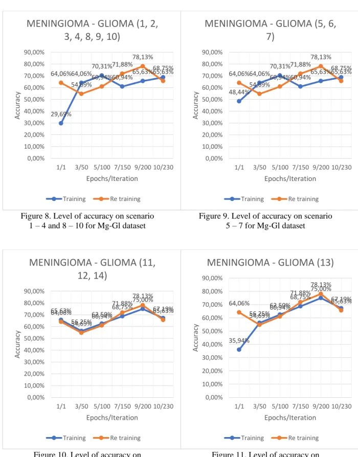
The structure of the CNN model for GLCM results using 1x1x1 input size and has 13 layers with 16 numfilters and [3 3] filter size. The test layer structure can be seen in Figure 6. The work process in this research using 4 combinations of brain tumor data which then done resize to form the same image size. After the dataset is formed, the training data is inserted into the Convolutional Neural Network so as to form the training model, the training model is retrained back to form a model ready for testing. The next stage is done testing to produce output of accuracy and time. Based on the number of combinations of datasets and test scenarios performed, fifty-six experiments were produced. The Processing Diagram of Brain Tumors Classification can be seen in Figure 7.

(6)

Figure 7. The Processing Diagram of Brain Tumors Classification

3. RESULTS AND DISCUSSION

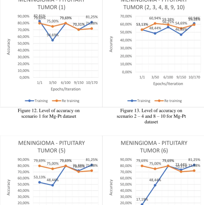
The training and retraining process on the Mg-Gl, Mg-Pt, Gl-Pt, and Mg-Gl-Pt datasets uses 14 combinations of GLCM features. The results of accuracy in training and retraining models with Mg-Gl datasets can be seen in Figures 8, 9, 10, and 11. Figure 8 shows that the training model has a lower accuracy than the retraining model in the early epoch, but in the 10th epoch the training model is superior to the retraining model with Ct, Cr, Eg, Hg, Cr-Eg, Cr-Hg, and Eg-Hg features. The same is shown in Figure 9. Figure 9 shows that the training model has a lower accuracy than the retraining model in the early epoch, but in the 10th epoch the training model is superior to the retraining model with Ct-Cr, Ct-Eg, and Ct-Hg features. Figure 10 shows that the training model has an accuracy similar to that of retraining in the early epoch until the 10th epoch with Ct-Cr-Eg, Ct-Cr-Hg, and Ct-Cr-Eg-Hg features. Figure 11 shows that the training model has a lower accuracy with the retraining model in the early epoch, but in the 10th epoch the training model has almost the same accuracy as the retraining model with Cr-Eg-Hg features.

The results of accuracy in training and retraining models with Mg-Pt datasets can be seen in Figures 12, 13, 14, 15, 16, 17, and 18. While the results of accuracy in training and retraining models with Gl-Pt datasets can be seen in Figures 19, 20, 21, 22, and 23.

Preprocessing Brain

Tumor

Image Resize Grayscale

Combination Feature of GLCM Dataset Training Retraining Model Testing

(7)

Figure 8. Level of accuracy on scenario 1 – 4 and 8 – 10 for Mg-Gl dataset

Figure 9. Level of accuracy on scenario 5 – 7 for Mg-Gl dataset

Figure 10. Level of accuracy on scenario 11, 12, 14 for Mg-Gl dataset

Figure 11. Level of accuracy on scenario 13 for Mg-Gl dataset

29,69% 64,06% 70,31% 60,94% 65,63% 68,75% 64,06% 54,69% 60,94% 71,88% 78,13% 65,63% 0,00% 10,00% 20,00% 30,00% 40,00% 50,00% 60,00% 70,00% 80,00% 90,00% 1/1 3/50 5/100 7/150 9/200 10/230 Acc u racy Epochs/Iteration

MENINGIOMA - GLIOMA (1, 2,

3, 4, 8, 9, 10)

Training Re training 48,44% 64,06% 70,31% 60,94% 65,63% 68,75% 64,06% 54,69% 60,94% 71,88% 78,13% 65,63% 0,00% 10,00% 20,00% 30,00% 40,00% 50,00% 60,00% 70,00% 80,00% 90,00% 1/1 3/50 5/100 7/150 9/200 10/230 Acc u racy Epochs/Iteration

MENINGIOMA - GLIOMA (5, 6,

7)

Training Re training 65,63% 56,25% 62,50% 68,75% 75,00% _67,19% 64,06% 54,69% 60,94% 71,88% 78,13% 65,63% 0,00% 10,00% 20,00% 30,00% 40,00% 50,00% 60,00% 70,00% 80,00% 90,00% 1/1 3/50 5/100 7/150 9/200 10/230 Acc u racy Epochs/Iteration

MENINGIOMA - GLIOMA (11,

12, 14)

MENINGIOMA - GLIOMA (13)

Training Re training

(8)

Figure 12. Level of accuracy on scenario 1 for Mg-Pt dataset

Figure 13. Level of accuracy on scenario 2 – 4 and 8 – 10 for Mg-Pt

dataset

82,81% 54,69% 79,69% 70,31% 81,25% 79,69% 75,00% 79,69% 70,31% 71,88% 0,00% 10,00% 20,00% 30,00% 40,00% 50,00% 60,00% 70,00% 80,00% 90,00% 1/1 3/50 6/100 9/150 10/170 Acc u racy Epochs/Iteration

MENINGIOMA - PITUITARY

TUMOR (1)

Training Re training 53,13% 48,44% 56,25% 46,88% 60,94% 53,13% 60,94% 59,38% 54,69% 59,38% 0,00% 10,00% 20,00% 30,00% 40,00% 50,00% 60,00% 70,00% 1/1 3/50 6/100 9/150 10/170 Acc u racy Epochs/Iteration

MENINGIOMA - PITUITARY

TUMOR (2, 3, 4, 8, 9, 10)

Training Re training 53,13% 48,44% 79,69% 71,88% 81,25% 79,69% 75,00% 79,69% 70,31% 71,88% 0,00% 10,00% 20,00% 30,00% 40,00% 50,00% 60,00% 70,00% 80,00% 90,00% 1/1 3/50 6/100 9/150 10/170 Acc u racy Epochs/Iteration

MENINGIOMA - PITUITARY

TUMOR (5)

MENINGIOMA - PITUITARY

TUMOR (6)

Training Re training

(9)

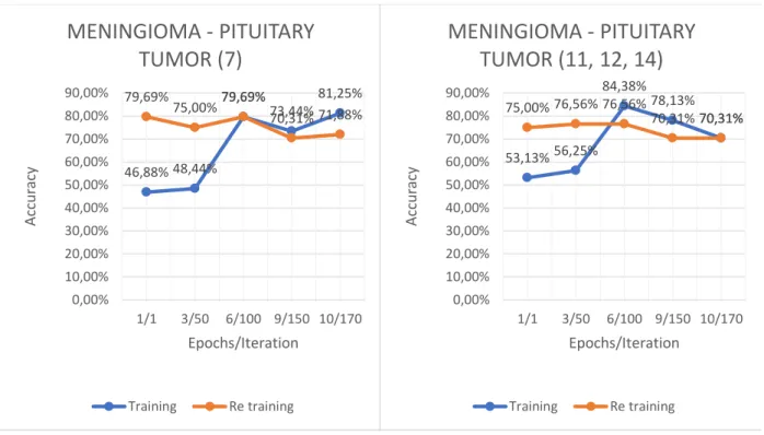
Figure 17. Level of accuracy on scenario 11, 12, 14 for Mg-Pt dataset

Figure 19. Level of accuracy on scenario 1, 6, 7 for Gl-Pt dataset

46,88% 48,44% 79,69% 73,44% 81,25% 79,69% 75,00% 79,69% 70,31% 71,88% 0,00% 10,00% 20,00% 30,00% 40,00% 50,00% 60,00% 70,00% 80,00% 90,00% 1/1 3/50 6/100 9/150 10/170 Acc u racy Epochs/Iteration

MENINGIOMA - PITUITARY

TUMOR (7)

MENINGIOMA - PITUITARY

TUMOR (11, 12, 14)

Training Re training 46,88% 56,25% 62,50% 40,63% 59,38% 53,13% 60,94% 59,38% 54,69% 59,38% 0,00% 10,00% 20,00% 30,00% 40,00% 50,00% 60,00% 70,00% 1/1 3/50 6/100 9/150 10/170 Acc u racy Epochs/Iteration

MENINGIOMA - PITUITARY

TUMOR (13)

Training Re training 70,31% 46,88% 82,81% 84,38% 84,38% 85,94% 75,00% 81,25% 82,81% 82,81% 81,25% 81,25% 0,00% 10,00% 20,00% 30,00% 40,00% 50,00% 60,00% 70,00% 80,00% 90,00% 100,00% Acc u racy Epochs/Iteration

GLIOMA - PITUITARY TUMOR

(1, 6, 7)

(10)

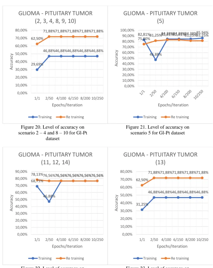
Figure 20. Level of accuracy on scenario 2 – 4 and 8 – 10 for Gl-Pt

dataset

Figure 21. Level of accuracy on scenario 5 for Gl-Pt dataset

Figure 22. Level of accuracy on scenario 11, 12, 14 for Gl-Pt dataset

Figure 23. Level of accuracy on scenario 13 for Gl-Pt dataset

29,69% 46,88% 46,88% 46,88% 46,88% 46,88% 62,50% 71,88% 71,88% 71,88% 71,88% 71,88% 0,00% 10,00% 20,00% 30,00% 40,00% 50,00% 60,00% 70,00% 80,00% 1/1 2/50 4/100 6/150 8/200 10/250 Acc u racy Epochs/Iteration

GLIOMA - PITUITARY TUMOR

(2, 3, 4, 8, 9, 10)

Training Re training 82,81% 46,88% 84,38% 84,38% 84,38% 85,94% 75,00% 81,25% 82,81% 82,81% 81,25% 81,25% 0,00% 10,00% 20,00% 30,00% 40,00% 50,00% 60,00% 70,00% 80,00% 90,00% 100,00% Acc u racy Epochs/Iteration

GLIOMA - PITUITARY TUMOR

(5)

GLIOMA - PITUITARY TUMOR

(11, 12, 14)

Training Re training 31,25% 46,88% 46,88% 46,88% 46,88% 46,88% 62,50% 71,88% 71,88% 71,88% 71,88% 71,88% 0,00% 10,00% 20,00% 30,00% 40,00% 50,00% 60,00% 70,00% 80,00% 1/1 2/50 4/100 6/150 8/200 10/250 Acc u racy Epochs/Iteration

GLIOMA - PITUITARY TUMOR

(13)

(11)

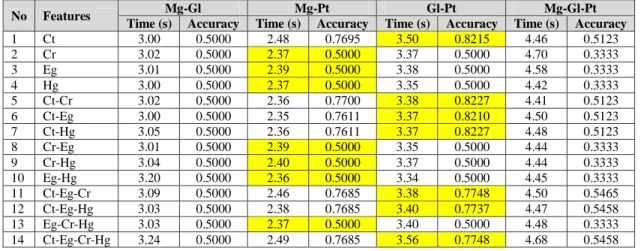
After doing this research, it is found that all test scenarios using Ct feature will increase accuracy more than 20%. For the data with the highest accuracy is in the data Gl-Pt with the accuracy of 82% and the test time for 3 seconds. The tumor data that does not use the accurate Ct feature will be the same. From this study it can be concluded that Ct is a feature that dominates with the highest accuracy on each combination of data which can be seen in Table 1.

Table 1 Overall Result Of Experiment With The Test And Dataset Scenario Combination

No Features Mg-Gl Mg-Pt Gl-Pt Mg-Gl-Pt

Time (s) Accuracy Time (s) Accuracy Time (s) Accuracy Time (s) Accuracy

1 Ct 3.00 0.5000 2.48 0.7695 3.50 0.8215 4.46 0.5123 2 Cr 3.02 0.5000 2.37 0.5000 3.37 0.5000 4.70 0.3333 3 Eg 3.01 0.5000 2.39 0.5000 3.38 0.5000 4.58 0.3333 4 Hg 3.00 0.5000 2.37 0.5000 3.35 0.5000 4.42 0.3333 5 Ct-Cr 3.02 0.5000 2.36 0.7700 3.38 0.8227 4.41 0.5123 6 Ct-Eg 3.00 0.5000 2.35 0.7611 3.37 0.8210 4.50 0.5123 7 Ct-Hg 3.05 0.5000 2.36 0.7611 3.37 0.8227 4.48 0.5123 8 Cr-Eg 3.01 0.5000 2.39 0.5000 3.35 0.5000 4.44 0.3333 9 Cr-Hg 3.04 0.5000 2.40 0.5000 3.37 0.5000 4.44 0.3333 10 Eg-Hg 3.20 0.5000 2.36 0.5000 3.34 0.5000 4.45 0.3333 11 Ct-Eg-Cr 3.09 0.5000 2.46 0.7685 3.38 0.7748 4.50 0.5465 12 Ct-Eg-Hg 3.03 0.5000 2.38 0.7685 3.40 0.7737 4.47 0.5458 13 Eg-Cr-Hg 3.03 0.5000 2.37 0.5000 3.40 0.5000 4.48 0.3333 14 Ct-Eg-Cr-Hg 3.24 0.5000 2.49 0.7685 3.56 0.7748 4.68 0.5458 4. CONCLUSIONS

Based on the results of brain tumor classification testing using Convolutional Neural Network, it can be concluded that all GLCM features combined with Contrast will improve accuracy. This shows that Contrast is a feature that dominates in the classification of brain tumors. In addition, two combined features that involve Contrast will get better accuracy than do not involve Contrast. The time difference from the accuracy results involving the Contrast feature in the classification process on a combination of brain tumor data is not very significant, but Contrast can raise 20% accuracy for all combinations of features involving Contrast.

REFERENCES

[1] D. Priyawati, I. Soesanti, and I. Hidayah, “Kajian Pustaka Metode Segmentasi Citra Pada MRI Tumor Otak,” Pros. SNST ke-6, Yogyakarta, 2016.

[2] I. W. S. E. Putra, A. Y. Wijaya, and R. Soelaiman, “Klasifikasi Citra Menggunakan Convolutional Neural Network (CNN) pada Caltech 101,” J. Tek. ITS, 2016.

[3] T. D. Vu, H.-J. Yang, V. Q. Nguyen, A.-R. Oh, and M.-S. Kim, “Multimodal learning using convolution neural network and Sparse Autoencoder,” Chonnam Natl. Univ., 2017. [4] C. Y. Aydo˘gdu, E. Albay, and G. Ünal, “Classification of brain tissues as lesion or

healthy by 3D convolutional neural networks,” Istanbul Tek. Üniversitesi, 2017.

[5] P. Moeskops, M. A. Viergever, A. M. Mendrik, L. S. de Vries, M. J. N. L. Benders, and I. Iˇsgum, “Automatic Segmentation of MR Brain Images With a Convolutional Neural Network,” IEEE Trans. Med. Imaging, 2016.

[6] S. S. M. Salehi, D. Erdogmus, and A. Gholipour, “Auto-context Convolutional Neural Network (Auto-Net) for Brain Extraction in Magnetic Resonance Imaging,” Harvard Med. Sch., 2017.

[7] J. Kleesiek et al., “Deep MRI brain extraction: A 3D convolutional neural network for

skull stripping,” Elsevier B.V, 2016.

(12)

segmentation in MRI using fully convolutional neural networks: A preliminary study,”

Univ. Minho, 2017.

[9] S. Pereira, A. Pinto, V. Alves, and C. A. Silva, “Brain Tumor Segmentation Using Convolutional Neural Networks in MRI Images,” IEEE Trans. Med. Imaging, 2016. [10] R. Lang, L. Zhao, and K. Jia, “Brain tumor image segmentation based on convolution

neural network,” Beijing Univ. Technol., 2016.

[11] M. N. Khasanah, A. Harjoko, and I. Candradewi, “Klasifikasi Sel Darah Putih Berdasarkan Ciri Warna dan Bentuk dengan Metode K-Nearest Neighbor (K-NN),”

IJEIS (Indonesian J. Electron. Instrum. Syst., vol. 6, no. 2, p. 151, 2016.

[12] X. Huang, X. Liu, and L. Zhang, “A Multichannel Gray Level Co-Occurrence Matrix for Multi/Hyperspectral Image Texture Representation,” Remote Sens, 2014.

[13] Clauditta, Lovidianti, D. Alamsyah, and Yohannes, “Menghitung Jumlah Orang dengan Ekstraksi Fitur Gray Level Co-occurrence Matrix (GLCM),” STMIK GI MDP Palembang, 2016.

[14] S. Goswami and L. K. P. Bhaiya, “A hybrid neuro-fuzzy approach for brain abnormality detection using GLCM based feature extraction,” Rungta Coll. Eng. Technol., 2013. [15] A. Chaddada, P. O. Zinnb, and R. R. Colena, “Radiomics texture feature extraction for

characterizing GBM phenotypes using GLCM,” Univ. Texas, 2015.

[16] A. M. Hasan and F. Meziane, “Automated screening of MRI brain scanning using grey level statistics,” Elsevier Ltd, 2016.