PROFITS AND POSITION CONTROL: A WEEK OF FX DEALING

(1)

P

ROFITS

A

ND

P

OSITION

C

ONTROL

:

A

W

EEK OF

FX

D

EALING

Richard K. Lyons U.C. Berkeley and NBER

This version: June 1997

Abstract

This paper examines foreign exchange trading at the dealer level. The dealer we track averages $100,000 in profits per day on volume of $1 billion per day (or one basis point). The half-life of the dealer’s position is only ten minutes, providing strong support for inventory models. A methodological innovation allows us to identify his speculative position over time. This speculative position determines the share of prof-its deriving from speculation versus intermediation: intermediation is much more im-portant.

Forthcoming, Journal of International Money & Finance. Correspondence

Professor Richard K. Lyons

Haas School of Business, U.C. Berkeley Berkeley, CA 94720-1900

Tel: 510-642-1059, Fax: 510-642-4700 E-mail: [email protected]

* I thank the following for helpful comments: Jeff Bohn, Frank Diebold, Bernard Dumas, Mark Flood, Dick Meese, Mark Ready, Andrew Rose, Patrik Säfvenblad, Matt Spiegel, Avanidhar Subrahmanyam, and seminar participants at Berkeley, UCLA, the Federal Reserve Board, the Federal Reserve Bank of New York, the NBER, and the Stockholm School of Economics. I also thank Jeff Bohn for valuable research assistance. Parts of this paper were written while visiting the IIES at Stockholm University and I thank them for their hospitality. Financial assistance from the National Science Foundation and the Berkeley Program in Finance is gratefully acknowledged.

(2)

P

ROFITS

A

ND

P

OSITION

C

ONTROL

:

A

W

EEK OF

FX

D

EALING

Empirical work on FX microstructure is still in its early stages. The earliest work used futures data since that was available at high frequencies.1 In FX, however, the futures market is both much smaller than spot and tightly linked to spot through arbitrage. Moreover, early data sets did not have sufficient granularity to capture agent heterogeneity, the hallmark of the microstructure approach. Work on the spot market itself grew in the early 90s with the availabil-ity of quotes on an intraday basis (specifically, the indicative quotes from Reuters called FXFX).2 These quotes provide a quite accurate picture of price dynamics. More important, they also speak to heterogeneity issues since the names and locations of the quoting banks are also included. A number of interesting questions could thus be addressed that earlier data did not permit. The FXFX data did not, however, leave much room for direct testing of theory since they provide no direct measures of quantity (order flow) — and quantity’s role in determining price is central to microstructure theory. As quantity data became available, more direct tests became possible.3

This paper extends earlier work by answering a number of key quantity-dependent questions. Answering some of these is rather straightforward. For example, how profitable is dealing in FX? And how rapidly do FX dealers dispose of risky inventory compared to, say, NYSE equity specialists? Other questions are less straightforward, requiring some methodologi-cal progress. For example, what share of dealer profits come from speculation versus intermedia-tion? To answer this, one needs a method for measuring dealer speculation over time. This paper introduces a method for doing this.

Our answers to the more straightforward questions are striking. First consider dealer profits: the dealer we track averages $100,000 profit per day (on volume of $1 billion per day). By comparison, equity dealers average about $10,000 profit per day (on volume of roughly $10

1

See for example Grammatikos and Saunders (1986). 2

See Goodhart and Figliuoli (1991) and Bollerslev and Domowitz (1993), among many others. At the

daily frequency, early work includes Glassman (1987) and Bossaerts and Hillion (1991). 3

See Lyons (1995), Goodhart, Ito, and Payne (1996), and Yao (1996). For an emerging experimental literature see Flood et al. (1996). For work on information networks embedded in FX trading technologies see Zaheer and Zaheer

(3)

million per day).4 Next, consider the pace of inventory management: the half-life for the dealer we track is only 10 minutes. This is remarkably short relative to half-lives for equity specialists of one week [Madhavan and Smidt (1993)]. Inventory theory is clearly essential to understanding trading in this market. Though striking, these results also present a challenge: Why do equity and FX markets look so different in these dimensions? That is a issue this paper raises, but does not resolve.

As stated above, addressing some of the less straightforward questions — e.g., the share of profits from speculation — requires some methodological progress. For perspective we turn to the relevant theory. Note that microstructure theory is composed of two distinct branches. The earlier branch of inventory models began in the 1970s.5 The later branch of information models developed in the 1980s.6 Underlying assumptions kept these branches distinct: inventory models include no information asymmetries, and information models include no inventory costs (e.g., no risk aversion). Consequently, a dealer’s position in inventory models is purely nonspeculative, while in information models it is purely speculative. In the data, of course, positions include both speculative and nonspeculative components. Disentangling them is an important step for empiri-cal work since theory is clear that the respective driving forces are different.

The methodological progress we make here is our means of disentangling speculative and nonspeculative positions. We are certainly not the first to effect this decomposition. The difference is that our approach draws from economics rather than being purely statistical [see Madhavan and Smidt (1993) and Hasbrouck and Sofianos (1993)]. Specifically, our method identifies the dealer’s speculative position by projecting his total position on an information set, one that contains non-public information useful for speculation. A second, crucial ingredient is that this information set is selected such that its contents are orthogonal to the dealer’s nonspecu-lative position. This instrumental-variables approach provides the identification we need.

In general, the information driving speculative positions comes from two key sources: incoming orders and incoming quotes. To drive speculation, it is important that this information not be public information, which it is not in this case: quantity and price information from FX

4

We use the numbers from Hansch et al. (1994) for the London Stock Exchange because, unlike the NYSE, this is a pure dealership market and therefore more comparable to FX. They find dealers average a profit of roughly 10 basis points on each transaction. Though the authors do not provide an average turnover by dealer, they do provide data that allow a rough estimate. The average daily turnover for FTSE-100 stocks is about $10 million (£6.9 million). This total turnover is divided among dealers, but active dealers make markets in many stocks. Given the market shares the authors report for the more active dealers, and given the number of stocks in which each makes markets, the estimated average turnover of $10 million per dealer is about right.

5

See Garman (1976), Amihud and Mendelson (1980), Ho and Stoll (1983), and O'Hara and Oldfield (1986), among others.

6

See Copeland and Galai (1983), Kyle (1985), Glosten and Milgrom (1985), and Admati and Pfleiderer (1988), among others.

(4)

dealer trades are not available to the market at large. [For more on this see Lyons (1996).] The first of these two sources, incoming orders, is the standard source of dealer information in information models. The second source, incoming quotes, is a special feature of multiple-dealer markets [see Leach and Madhavan (1993)].7 In fact, our position decomposition would not be possible without this feature: in single-dealer models there is typically a single determinant of both speculative and nonspeculative positions — namely order flow — and a single determinant cannot serve as an instrument for disentangling these two position components; with multiple-dealers, however, incoming quotes provide a second determinant of speculative position, one that may be uncorrelated with non-speculative position, and can therefore serve as an instrument.

Performing the decomposition allows us to pin down the degree to which profit is due to intermediation (i.e., the spread) versus speculative gains. We find that intermediation, at least for the dealer we track, is much more important, accounting for roughly 90 percent of his profits. To this we should add, however, that our dealer is described by his peers as a “liquidity machine,” by which they mean that his style focuses on high volume at competitive prices. In addition, more that 90 percent of our dealer’s trading is with other dealers (as opposed to non-dealer customers), whereas the average interdealer share is closer to 80 percent. Thus, in terms of the source of his profits, our dealer should not be viewed as representative of all dealers in this market.8

Though many empirical papers address dealer behavior, two are especially relevant here due to their focus on quantity data. Each examines implications of microstructure models using data on equity specialist inventories. Madhavan and Smidt (1993) use their inventory data to test whether inventories revert toward a target (as predicted by the theory). Their model of the target to which inventory reverts is statistical, based on systematic patterns in residuals. They find that allowing the target to vary intensifies mean reversion. Nevertheless, the shortest half-life they estimate is one week. Hasbrouck and Sofianos (1993) also focus on the inventory series itself. And their model of target inventory is also statistical, in this case driven by inventory’s time-series properties.9 Like Madhavan and Smidt (1993), they find allowing the target to vary helps account for earlier findings that inventory control is weak.

Before proceeding we want to clarify our terms, in particular our use of “position

7

It could be argued that limit orders play a similar role within specialist markets. 8

See, for example, Yao (1996), who chronicles the trading of a commercial bank dealer who receives much more customer order flow than our dealer.

9

The three time-series properties of inventory highlighted by Hasbrouck and Sofianos (1993) are short-term variation, discrete long-term variation, and smooth long-term variation (page 1570). Their view is that the short-term variation reflects classic dealer behavior (nonspeculation) whereas long-term variation of both types reflects investment holdings (speculation). The position series for an FX dealer displays only short-term variation by their standards since in general the daily closing position is zero. Thus, by their logic our position series must be devoid of any speculative

(5)

compo-control.” Here position control refers to management of both speculative and nonspeculative positions. The more traditional term “inventory control” is narrower, referring only to manage-ment of nonspeculative positions. Since this paper’s scope spans both, we adopt a more flexible terminology.

The paper is organized as follows: The next section outlines our method for disentangling speculative and nonspeculative positions; Section II describes the data; Section III disentangles the position components and estimates dealer profits; Section IV concludes.

(6)

I. Decomposing Speculative and Nonspeculative Position Components

I.A. Linking Target Position to Information

Consider the equation used by Madhavan and Smidt (1993) to estimate mean reversion in dealer positions (our appendix sketches the optimizing model underlying it):

(1)

I

_t₊₁

−

I

_t

=

β

(

I

_t

−

I

_t∗

)

+

ε

_t₊₁

where

I

_t is the dealer's total position, and

I

_t∗ is the dealer's target position, both at time t. The position disturbance ε_t+1 is realized at t+1 and is uncorrelated with

I

_t-

I

_t∗ (a property deriving from the assumption that quotes are regret-free in the sense of Glosten and Milgrom (1985)). The difficulty in estimating β comes from the unobservability of

I

_t∗. Since most models specify order flow as the only source of variation in both

I

t and

I

t

∗

, it is impossible to identify

I

t

∗

on the basis of order flow alone, hence the past reliance on statistical models of

I

t

∗

.

We need to be precise about the term target position. The dealer's target position can be decomposed into a speculative demand component

I

t

s

and a nonspeculative component

I

t n ∗ . (2)

I

t

I

t

I

s t n ∗

=

+

∗

For an FX dealer, it is reasonable to presume that

I

t n

∗

equals zero. In particular, it is unclear why a non-zero nonspeculative position would aid a major-market FX dealer in the provision of immediacy (e.g., an FX dealer does not worry about stock-out as he might in a less liquid mar-ket). Also supportive is the fact that FX dealers generally close each day with a position of zero (unlike NYSE specialists). Under the assumption that

I

t

n

∗

equals zero, we can therefore write:

(3)

I

_t₊₁

−

I

_t

=

β

(

I

_t

−

I

_ts

)

+

ε

_t₊₁

Note that we are not assuming the nonspeculative component of total position

I

_t is zero, only that the nonspeculative component of the target position is zero. Accordingly, we decompose the total position at any time t into speculative and nonspeculative components:

(7)

(4)

I

_t

=

I

_ts

+

I

_tn

where

I

_tn denotes the time t nonspeculative component.

The speculative component is the dealer's speculative demand which we model in the usual way [see O’Hara (1995), pages 156-158)]. The demand for the risky asset in a competitive two-asset economy, one riskless and one risky, with utility defined over end-of-period wealth is:

(5)

I

_ts

=

θ

E P

[

_t₊₁

−

P

_t

Ω

_t

]

where P_t is the price of the risky asset (FX) at time t, Ω_t is the dealer's information set at time t, and θ is a constant. The constant θ depends on the coefficient of absolute risk aversion and the conditional variance of the risky asset price. For now, we assume a constant conditional variance, though we return to this issue below.

I.B.. Consistent Estimation of β

The usual difficulty in extracting

I

_ts from

I

_t is due to the correlation between

I

_ts and

I

_tn. To see this, consider the canonical specialist who draws inferences about the risky asset's value from the incoming order flow. In this context, incoming order flow is driving both

I

_tn and

I

_ts, the latter due to order flow’s information content. Consequently, order flow alone is insuffi-cient for disentangling these two components of

I

_t. Instruments are needed for

I

_ts: variables correlated with

I

_ts but uncorrelated with

I

_tn.

A richer specification of Ω_t provides the needed instruments. Partition Ω_t into three components: (i) a set of public signals

Ω

_tP, (ii) a set of non-public signals correlated with

I

_tn, or

Ω

_tN

, and (iii) a set of non-public signals orthogonal to

I

_tn, or

Ω

_tN⊥:

(6)

Ω

_t

=

{

Ω Ω Ω

_tP

,

_tN

,

_tN⊥

}

The least-squares projection of

I

_t on

Ω

_tN⊥ is thus purged of any correlation with inventory changes due to

I

_tn. Let

I

$

_ts denote this projection. We can then consistently estimate the half-life of the nonspeculative position component from:

(8)

(7)

I

_t₊₁

−

I

_t

=

β

(

I

_t

−

I

$

_ts

)

+

ε

_t₊₁

since

I

$

_ts is by construction orthogonal to ε_t+1. This is the mean reversion we associate with inventory control in the classic models.

I.C. A Consistent Covariance Matrix of

β

$

Though an OLS estimate of from Eq. (7) is consistent, the OLS standard errors are incorrect. To see this, define the projection error of

I

$

_ts as η_t.

(8)

I

$

_ts

=

I

_ts

+

η

_t

If we denote the variance of the disturbance from Eq. (3) as

σ

_ε2, then the variance of the distur-bance in Eq. (7) is

σ

_ε2 +

β σ

2 _η2. The probability limit of the OLS estimate of the residual covariance matrix from Eq. (7) is

σ

_ε2, which clearly understates the asymptotic standard errors. Pagan (1984) shows that Two-Stage Least Squares (2SLS) produces a consistent estimator of the variance of

β

$. This is the estimator we use to calculate standard errors for estimates of Eq. (7).

II. Data

The dataset is an augmented version of that used in Lyons (1995), the principal addition being the non-dealt quotes we use to identify the dealer’s speculative position. Here we provide a broad overview, with detail only where necessary to augment that in Lyons (1995).

The dataset consists of two linked parts, each covering the activity of a DM/$ dealer at a major New York bank. The sample spans the five trading days of the week August 3-7, 1992. Each of the five trading days begins at 8:30 A.M. and ends on average at 1:30 P.M., Eastern Standard Time. The first part comprises the dealer's position cards. His position cards include all his trades, with transaction quantities and prices. The second part is narrower but deeper: nar-rower because it contains only a subset of his trades, his direct (meaning non-brokered)

(9)

inter-dealer trades; deeper because it contains all his direct quotes, irrespective of whether dealt. Figure 1 provides a diagram of the data flow through time.

II.A. Dealer Data: Position Cards

Because the position cards include all of the dealer's transactions, they are sufficient for constructing the dealer's position

I

t through time. An average day consists of approximately 20 cards, each with about 15 transaction entries. Each card includes the following information for every trade:

(1) the signed quantity traded (which determines

I

_t) (2) the transaction price

(3) the counterparty, including whether brokered.

Note that the bid/ask quotes at the time of the transaction are not included on the position sheets. Note also that each entry is not time-stamped, though the dealer does record the time at the outset of every card (to the minute), and occasionally within the card too. This part of the dataset includes 1720 transactions amounting to $7.0 billion. Figure 2 provides a diagram of the position sheet's structure. The only dimension of an actual position sheet that is not in the diagram is the names of the counterparties. Counterparty names are considered highly confidential to this dealer's institution.

II.B. Dealer Data: Direct Quotes and Trades

The second part of the dataset includes the quotes, transaction quantities, and transaction prices for all the non-brokered interdealer interactions. These data derive from bank dealing records from the Reuters Dealing 2000-1 system. This system is different from the system that produces the Reuters FXFX indications used elsewhere in the literature [see, for example, Goodhart and Figliuoli (1991)]. It allows dealers to communicate quotes and trades bilaterally via computer rather than verbally over the telephone. This dealer uses Dealing 2000-1 for more than 99% of his non-brokered interdealer trades.

(10)

Each record from the Dealing 2000-1 system includes the first 5 of the following 7 variables. The last two are included only if a trade takes place.

(1) The time the communication is initiated (to the minute, with no lag) (2) which of the two dealers is requesting the quote

(3) the quote quantity (4) the bid quote (5) the ask quote (6) the quantity traded (7) the transaction price.

This part of the dataset includes 952 transactions amounting to $4.1 billion. Though it does not include the dealer's brokered transactions, it has two key advantages over the data from the position cards: it provides quotes rather than just transaction prices and it identifies which counterparty is the aggressor. It also provides a means of error-checking the data from the position cards. Perhaps most important for our purposes, this part of the dataset provides the incoming quotes that did not generate a trade. We use these non-dealt quotes to identify the dealer’s speculative position. Over our sample week, only 5 percent of incoming quotes gener-ated a trade. (In contrast, 34 percent of outgoing quotes genergener-ated a trade, an indication that our dealer is not the average dealer in this respect.)

II.C. The Resulting Position Series

Figure 3 provides a plot of the dealer's position over the sample's five trading days. Mean reversion is evident. Note too the range of the position: rarely did open positions rise above $40 million ($40 million is well below the intraday position limits imposed on senior dealers at major banks, typically in the $100-$150 million range). Each of the five days the dealer closed his trading day with a position of zero. (A common overnight limit is about $75 million; most dealers, however, close their day at zero. Two common rationales for closing at zero are that (1) carrying an open position requires monitoring it through the evening and (2) a dealer’s

(11)

compara-tive advantage in speculation is when she is seated at her desk observing order flows and quotes.) The relative width of the days is a reflection of the relative trading activity. Monday and Friday are the highest volume days.

III. Results: Profits and Position Components

III.A. Dealer Profits

A summary of the dealer's profitability over the week appears in Table 1. Note that the daily volume is well over $1 billion each day. Profits for the week total $507,929, Friday being the most profitable day. Friday is also the highest volume day. Of course, if profits derive primarily from speculative positions, then volatility is more important than volume. Friday also has the highest volatility in the five-day sample.

We turn now to the question of whether profits tend to come from intermediation or speculation. As a first step, we impute the intermediation component of profits using an assump-tion that the dealer himself felt is reasonable. Specifically, we assume that the cost of laying off an incoming order is one-third of the dealer’s bid-ask spread. For example, if the dealer quotes his median spread of three pips at DM 1.4750/$ - DM 1.4753/$ and the incoming order is a purchase of dollars at DM 1.4753/$, then on average the dealer must provide price improvement on the bid side of DM 1.4751 to induce an offsetting customer sale. This translates into an average profit of one pip on every transaction.

The results appear in the “Profit: Spread” column of Table 1. The profits imputed to in-termediation correspond quite closely to total profits: the two differ by less than 10 percent. Given the dealer himself feels the assumption driving this comparison is reasonable, intermedia-tion appears to be a much more important source of profits. Still, to get a more complete picture, we need to examine whether his speculative positions are profitable.

III.B. Position Decomposition

Per section I, disentangling the speculative and nonspeculative position components requires instruments that are correlated with the speculative component but uncorrelated with the nonspeculative component. The instrument sets we consider rely exclusively on non-dealt,

(12)

incoming quotes (specifically, lagged changes).10 These quotes are not public information, so they are arguably relevant for speculative position taking. On the other hand, they are do not produce a transaction, so there is no direct relation to the nonspeculative component of our dealer’s position. Of course, no direct relation does not rule out an indirect relation. One ration-ale for ruling out even an indirect relation is embedded in the model of Lyons (1997). In that model, past price change is orthogonal to nonspeculative position because dealers — being risk averse — set price to avoid nonspeculative positions; though nonspeculative positions still arise, optimal use of past information brings the correlation with price to zero.

Nevertheless, incoming quote changes cannot identify the speculative component

I

_ts if they are uncorrelated with the dealer's total position. Column two of table 2 (rows 2-4) verifies that these instruments are indeed correlated with

I

_t.11 The R2's indicate that

I

$

_ts, which is the projection of

I

_t on the information set Ω, accounts for about one-quarter of the variation in the dealer's total position. Put differently, Ω contains information useful to the dealer in determining his speculative demand. The first row of the table is included as a benchmark. With an empty information set, it is equivalent to assuming that target position

I

$

t

s

equals zero. (Hence, there is no first stage projection, and the R2 is not applicable.)

Table 2 also presents estimates of the half-life of nonspeculative positions.12 A half-life of ten minutes is extremely short relative to the position half-lives estimated in equity markets; for example, the lowest estimate for equity specialists in Madhavan and Smidt (1993) is 7 days. Our finding of ten minutes is clear evidence of aggressive inventory control. Of course, the FX market is not the NYSE. Why they trade so differently, however, is still an open question. Results like this reinforce the fact that the FX market is distinctive at the microstructural level.

10

In our data set, typically incoming quotes do not elicit a transaction: more than 80 percent of incoming quotes lapse without a deal. This large share of “non-dealt” quotes suggests that dealers gather quotes because they are informative, not simply because they provide immediacy.

For lack of data, previous work has had to identify no-trade “events” as the elapsing of a given amount of time without a transaction [e.g., five minutes in Easley, Kiefer, and O’Hara (1997)]. An important strength of our data set is that it includes non-dealt events explicitly.

11

The last of the three information sets — row 4 of Table 2 — includes a squared lagged price change in addition to the signed lagged price changes. Though this can only improve the first-stage fit, the orthogonality of this variable is more difficult to defend on theoretical grounds.

12

(13)

III.C. Regression Diagnostics

Some regression diagnostics are in order. First, there is no evidence of serial correlation (Durbin-Watson and Ljung-Box Q tests) or heteroskedasticity (White test). A natural next step is to examine structural stability, in particular, with respect to time-of-day. To do so, we split the sample into two subsamples, early and late, where early is defined as all observations occurring before the midpoint of the trading day (median transaction time). A Wald test of the equality of

$

β

across the two subsamples is rejected at the one percent level. Clearly, time-of-day is related to inventory control, which is not surprising given the dealer starts and ends each day with a zero net position.

To capture this time-of-day effect, we include an additional term in the model of Eq. (1):13

(9)

I

_t₊₁

−

I

_t

=

β

₁

(

I

_t

−

I

$

_ts

)

+

β

₂

(

%

Day

_t

)

(

I

_t

−

I

$

_ts

)

+

ε

_t₊₁

where the proxy “

%

Day

_t” is defined over each day as (observation #, day n) divided by (total # observations, day n), with n=1,...,5.14 The results appear in Table 3. Note that the time-independent component of mean reversion is insignificantly different from zero (

β

$₁). In contrast, the time-dependent component,

β

$₂, now does all the work. The estimates imply that the time-dependent component of mean reversion moves from zero at the start of each day to about -0.3 at the end. The implied half-lives at three points within the dealer's day appear in the last columns. On the whole, this time profile squares nicely with the fact that FX dealers typically close their positions at the end of each trading day.

Another important consideration is the impact of price volatility on the pace of mean reversion. It is not a priori clear, however, how volatility should affect mean reversion. On one hand, the higher volatility, the greater the benefit of inventory control. On the other hand, the higher volatility, the greater the cost of inventory control (spreads at brokers widen, as do direct spreads quoted by other dealers; for some evidence from indicative quotes, see Bessembinder

13

Note that while Eq. (1) is derived from an optimizing model, the same cannot be said of our adjustments to it. The technical challenge of doing so is formidable, and the payoff, in our judgment, marginal.

14

We refer to this as a proxy because the denominator—total transactions for the day—is not known to the dealer in advance.

(14)

(1994) and Bollerslev and Melvin (1994)). To capture this, we estimate the following linear model:

(10)

I

_t₊₁

−

I

_t

=

β

₁

(

%

Day

_t

)

(

I

_t

−

I

$

_ts

)

+

β

₂

(

HighVol

_t

)(

%

Day

_t

)

(

I

_t

−

I

$

_ts

)

+

ε

_t₊₁

where the dummy variable “

HighVol

_t” is equal to one if

(

∆

P

_t₋₁

)

2 is above its median, zero otherwise. The first regressor is the same as the second regressor in the model of Eq. (9) (recall that the first regressor in Eq. (9) produced an insignificant coefficient). The results appear in Table 4. The coefficient

β

$₂ is significant at the five percent level but not at one percent. The size and sign of

β

$₂ imply that mean reversion is lower when volatility is high. This suggests that when volatility increases, the added cost of inventory control dominates the added benefit. The implied half-lives at high and low volatility appear in the last columns (calculated at %Day=50%). The half-life is about twice as long with high volatility than with low volatility.

III.D. Profits From Speculative Component

Though section III.A. provides estimates of profit from intermediation, our measure of the dealer’s speculative position allows us to estimate speculative profit directly. We proceed in two stages. First, we determine whether the dealer’s speculative position forecasts future price changes. In particular, we test whether speculative position Granger causes price changes. Though not a sufficient condition for profitable speculation, the result provides useful perspec-tive. Then, in stage two, we mark the speculative position to market using the midpoint of the incoming quote closest to the measured speculative position change. The accumulated changes in net value provide an estimate of speculative profit. (Unlike our exact measure of total profit in Table 1, it is not possible to calculate speculative profit exactly since our measured changes in speculative position are not linked one-for-one with market transactions.)

On both counts, our results do not evince speculative profits. We find no evidence of Granger causality running from speculative position to prices. Further, even using quote mid-points, the speculative position does not generate profits; in fact, over the week the dealer suffered negligible losses on the speculative position. It is important to keep in mind, however,

(15)

that we are working with only one week of data, which may not be representative with respect to speculative profits. To be sure, speculative profits are much more volatile than profits from intermediation.

IV. Conclusions

We are able to address a number of questions that have not yet been examined in empiri-cal work on FX microstructure. And our answers to these questions are striking. First the dealer we track is quite profitable: he averages $100,000 profit per day (on volume of $1 billion per day). By comparison, equity dealers average about $10,000 profit per day (on volume of roughly $10 million per day). Second, we also find quite rapid inventory management: the half-life for the dealer we track is only 10 minutes. This is remarkably short compared to half-lives for equity specialists of one week. Why do equity and FX markets generate such different results at the microstructural level? This is an important topic for future research.

The paper also makes methodological progress. Specifically, we develop a method for measuring speculative position-taking over time. Unlike past — purely statistical — methods for doing this, our measure is based on the information flows that drive speculation. We use this measure of speculative position to pin down the extent to which dealer profits derive from speculation. In the end we find that intermediation is much more important source of profits, at least for the dealer we track over the week we are able to track him.

(16)

Appendix

Sketch of Madhavan and Smidt (1993) Derivation of Eq. (1) Agents: (1) Risk neutral informed trader

(2) Liquidity traders

(3) Risk neutral dealer, with inventory carrying costs (proportional to the variance of wealth)

Preferences: The dealer and informed trader maximize the expected value of terminal wealth. Liquidity trader preferences are not modeled (their trading can be generated as optimizing in the context of endowment shocks).

Market: There is a single risky asset that trades in a series of auctions. There is a constant probability (1-ρ) that a given time τ will be the liquidation time. The asset's fun-damental value follows a random walk. This value is known by the informed trader.

Notation: ν_t : fundamental value at time t

µ_t : dealer's conditional expectation of ν_t Ω

t : dealer's information set

W_t : dealer's wealth I_t : dealer's position P_t : price

z_t : excess demand, a function of P_t

Q_t : demand of informed trader, a function of P_t

X_t : demand of liquidity traders (aggregate), not a function of P_t D_t : intercept of demand schedule, informed plus uninformed

The informed trader's demand is proportional to the gap between fundamental value and price.

(A1)

Q v P

t

(

t

,

t

) (

=

δ

v

t

−

P

t

)

It is helpful to define the intercept of the excess demand schedule as the following:

(A2)

D

_t

=

δ

v

_t

+

X

_t

When divided by δ, this variable D_t provides an unbiased signal of the fundamental value ν_t (since X_t is mean zero).

(A3)

D

_t

δ

=

v

_t

+

X

_t

δ

Now, the updating equation can be expressed as a weighted average of this signal and the dealer's prior expectation.

(17)

(A4)

µ

_t

=

φ

(

D

_t

δ

) (

+ −

1

φ µ

)

_t₋₁

This evolution of the dealer's expectation can then be integrated with the dealer's stochastic programming problem. (A5)

[

]

[

]

P j j j t

Max

E W

Ω

j

= ∞

∑

=

1

Pr

τ

The solution to this stochastic programming problem yields Eq. (1) in the text: (1)

I

_t₊₁

−

I

_t

=

β

(

I

_t

−

I

_t∗

)

+

ε

_t₊₁

where the error term in the regression corresponds to the dealer's estimate of liquidity-trader demand X_t in the model:

(A6)

ε

t+

( )

β

E X

[

t t

]

+

≡ −

1 1 2

Ω

(18)

References

Admati, A. and Pfleiderer, P. (1988) A theory of intraday patterns: Volume and price variability.

Review of Financial Studies1, 3-40.

Amihud, Y. and Mendelson, H. (1980) Dealership market: Market making with inventory.

Journal of Financial Economics8, 31-53.

Ammer, J. and Brunner, A. (1994) Are banks market timers or market makers? Explaining foreign exchange trading profits. International Finance Discussion Paper #484, Board of Governors of the Federal Reserve System.

Bessembinder, H. (1994) Bid-ask spreads in the interbank foreign exchange market. Journal of

Financial Economics35, 317-348.

Bollerslev, T. and Domowitz, I. (1993) Trading patterns and prices in the interbank foreign exchange market. Journal of Finance48, 1421-1444.

Bollerslev, T. and Melvin, M. (1994) Bid-ask spreads and volatility in the foreign exchange market: An empirical analysis. Journal of International Economics36, 355-372.

Bossaerts, P. and Hillion, P. (1991) Market microstructure effects of government intervention in the foreign exchange market. Review of Financial Studies4, 513-541.

Copeland, T. and Galai, D. (1983) Information effects on the bid-ask spread. Journal of Finance

38, 1457-1469.

Easley, D., Kiefer, N. and O'Hara, M. (1997) One day in the life of a very common stock. Review

of Financial Studies, forthcoming.

Flood, M. (1992) Market structure and inefficiency in the foreign exchange market. Journal of

International Money and Finance13, 131-158.

Flood, M., Huisman, R., Koedijk, K. and Mahieu, R. (1996) Price discovery in multiple-dealer financial markets: The effect of pre-trade transparency. Concordia University typescript, December

Garman, M. (1976) Market microstructure. Journal of Financial Economics3, 257-275.

Glassman, D. (1987) Exchange rate risk and transactions costs: Evidence from bid-ask spreads.

Journal of International Money and Finance6, 479-490.

Glosten, L. and Milgrom, P. (1985) Bid, ask, and transaction prices in a specialist market with heterogeneously informed agents. Journal of Financial Economics14, 71-100.

Goodhart, C. and Figliuoli, L. (1991) Every minute counts in financial markets. Journal of

(19)

Goodhart, C., Ito, T. and Payne, R. (1996) One day in June 1993: A study of the working of the Reuters 2000-2 electronic foreign exchange trading system. In The Microstructure of

For-eign Exchange Markets, eds. J. Frankel, G. Galli and A. Giovannini, pp. 107-179.

Univer-sity of Chicago Press, Chicago, IL.

Grammatikos, T. and Saunders, A. (1986) Futures price variability: A test of maturity and volume effects. Journal of Business59, 319-330.

Hansch, O., Naik, N. and Viswanathan, S. (1994) Trading profits, inventory control and market share in a competitive dealer market. Duke University typescript, November.

Hasbrouck, J. (1988) Trades, quotes, inventories, and information. Journal of Financial Econom-ics22, 229-252.

Hasbrouck, J. and Sofianos, G. (1993) The trades of market makers: An empirical analysis of NYSE specialists. Journal of Finance48, 1565-1593.

Ho, T. and Stoll, H. (1983) The dynamics of dealer markets under competition. Journal of

Finance38, 1053-1074.

Kyle, P. (1985) Continuous auctions and insider trading. Econometrica53, 1315-1335.

Leach, J. and Madhavan, A. (1993) Price experimentation and security market structure. Review

of Financial Studies6, 375-404.

Lyons, R. (1995) Tests of microstructural hypotheses in the foreign exchange market. Journal of

Lyons, R. (1996) Optimal transparency in a dealer market with an application to foreign ex-change. Journal of Financial Intermediation5, 225-254.

Lyons, R. (1997) A simultaneous trade model of the foreign exchange hot potato. Journal of

International Economics42, 275-298.

Madhavan, A. and Smidt, S. (1991) A bayesian model of intraday specialist pricing. Journal of

Madhavan, A. and Smidt, S. (1993) An analysis of changes in specialist inventories and quota-tions. Journal of Finance48, 1595-1628.

O'Hara, M. (1995) Market Microstructure Theory. Blackwell Business, Cambridge MA.

O'Hara, M. and Oldfield, G. (1986) The microeconomics of market making. Journal of Financial

and Quantitative Analysis21, 361-376.

Pagan, A. (1984) Econometric issues in the analysis of regressions with generated regressors.

International Economic Review25, 221-247.

Yao, J. (1996) Market making in the interbank foreign exchange market, New York University typescript, December.

(20)

Zaheer, A. and Zaheer, S. (1995) Catching the wave: Alertness, responsiveness, and market influence in global electronic networks. University of Minnesota typescript, December.

(21)

Table 1

Summary of DM/$ dealer's trading and profits from Monday, August 3 to Friday, August 7, 1992.

The “$ Profit: Spread” column reports the profit the dealer would have realized if he had cleared one-third of his spread on every transaction. It is calculated as the dollar volume times one-third the median spread he quoted in the sample (median spread = DM 0.0003/$), divided by the average DM/$ rate over the sample (DM 1.475/$).

Transactions Volume (mil) Profit: Actual Profit: Spread

Monday 333 $ 1,403 $ 124,253 $ 95,101 Tuesday 301 $ 1,105 $ 39,273 $ 74,933 Wednesday 300 $ 1,157 $ 78,575 $ 78,447 Thursday 328 $ 1,338 $ 67,316 $ 90,717 Friday 458 $ 1,966 $ 198,512 $ 133,298 Total 1,720 $ 6,969 $ 507,929 $ 472,496

(22)

Table 2

Mean Reversion in Dealer Positions

(

)

I

t

I

t

I

t

I

t s

t

+1

−

=

β

−

$

+

ε

+1

Definitions:

I

t+1 is the dealer's position following the incoming trade at time t+1, where each

incoming trade in the sample defines a single period (i.e., transaction time).

I

$

t s

is an estimate of the dealer's speculative position at time t, defined as a projection on an information set Ω. The information sets we consider appear in column one.

∆

P

t,5 is the cumulative change in the

nondealt quotes received by the dealer over the period spanning five incoming trades prior to the incoming trade at t. Note that the first of the information sets implies

I

$

t

s

=0. The error term

ε

t+1

represents disturbances to the dealer's position from the provision of immediacy. Estimation: First, we estimate

I

$

t

s

as the OLS projection of

I

t on

Ω

. Then, we use

I

$

t s

to estimate

β

from the above equation using OLS. Column two presents the R2's from the projec-tion of

I

_t on

Ω

. In rows 2-4, the t-statistics in parentheses are calculated from 2SLS standard errors to account for the use of a generated regressor. The implied half-life is calculated as the mean intertransaction time (1.8 minutes) times the half-life in transactions implied by

β

$ [defined as -ln(2)/ln(1+

β

$)].

Sample: 838 observations from Monday, August 3 to Friday, August 7, 1992.

Information set R2 of projection

β

$ Implied half-life

{ }

Ω =

N.A. -0.10 (-5.63) 12 minutes

{ }

Ω

=

∆

P

_t,5 0.24 -0.12 (-5.73) 10 minutes

{

}

Ω

=

∆

P

_t_,₅

,

∆

P

_t₋_{5 5}_, 0.26 -0.12 (-5.64) 10 minutes

{

}

Ω

=

∆

P

t,5

,

∆

P

t₋5 5,

, (

∆

P

t,5

)

2 0.29 -0.13 (-5.97) 9 minutes

(23)

Table 3

Time-Dependent Mean Reversion in Dealer Positions

(

)

(

)

(

)

I

t

I

t

I

t

I

t

Day

I

s t t t s t +1

−

=

β

1

−

$

+

β

2

%

−

$

+

ε

+1

Definitions:

I

$

t s

is an estimate of the dealer's speculative position at time t, defined as a projection on an information set Ω. The information sets we consider appear in column one.

∆

P

nondealt quotes received by the dealer over the period spanning five incoming trades prior to the incoming trade at t. The variable “

%

Day

t” is defined over each day as (observation #, day n)/(total # observations, day n), n=1,...,5. The error term ε_t+1 represents disturbances to the dealer's position from the provision of immediacy.

Estimation: First, we estimate

I

$

t s

as the OLS projection of

I

t on Ω. Then, we use

I

$

t s

to estimate

β

from the above equation using OLS. The t-statistics in parentheses are calculated from 2SLS standard errors to account for the use of a generated regressor. The three half-life columns report the implied half-life when the dealer's day (%Day) is 25% done, 50% done, and 75% done. The implied half-life is calculated as the mean intertransaction time (1.8 minutes), times the half-life in transactions implied by

β

$₂ [defined as -ln(2)/ln(1+

β

$₂)], times “

%

Day

_t”.

Implied half-life Information set

β

$ 1

β

$2 25% 50% 75%

{ }

Ω

=

∆

P

t,5 0.02 (0.29) -0.30 (-3.06) 16 8 5 minutes

{

}

Ω

=

∆

P

_t_,₅

,

∆

P

_t₋_{5 5}_, 0.03 (0.46) -0.32 (-3.13) 16 7 5 minutes

(24)

Table 4

The Impact of Volatility on Time-Dependent Mean Reversion in Dealer Positions

(

)

(

)

(

)(

)

(

)

I

t

I

t

Day

t

I

t

I

t

HighVol

Day

I

s

t t t t

s t

+1

−

=

β

1

%

−

$

+

β

2

%

−

$

+

ε

+1

Definitions:

I

$

t s

is an estimate of the dealer's speculative position at time t, defined as a projection on an information set

Ω

. The information sets we consider appear in column one.

∆

P

nondealt quotes received by the dealer over the period spanning five incoming trades prior to the incoming trade at t. The variable “

%

Day

t” is defined over each day as (observation #, day n)/(total # observations, day n), n=1,...,5. The dummy variable “

HighVol

t” is equal to one if

(

∆

P

t−1

)

2

is higher than its median, zero otherwise. The error term

ε

t+1 represents disturbances to

the dealer's position from the provision of immediacy.

Estimation: First, we estimate

I

$

_ts as the OLS projection of

I

_t on

Ω

. Then, we use

I

$

_ts to estimate

β

from the above equation using OLS. The t-statistics in parentheses are calculated from 2SLS standard errors to account for the use of a generated regressor. The two half-life columns report the implied half-life when the dealer's day is 50% done and volatility is high (

HighVol

_t=1) and low (

HighVol

_t=0). The implied half-life is calculated as the mean inter-transaction time (1.8 minutes), times the half-life in inter-transactions implied by

β

$₁ and

β

$₂[defined as -ln(2)/ln(1+

β

$), where

β

$=

β

$₁ with low volatility and

β

$=

β

$₁+

β

$₂ with high volatility], times 0.5 to account for “

%

Day

_t”.

Implied half-life

Information set

β

$

1

β

$2 High Vol. Low Vol.

{ }

Ω

=

∆

P

t,5 -0.36 (-4.56) 0.21 (2.09) 13 6 minutes

{

}

Ω

=

∆

P

_t_,₅

,

∆

P

_t₋_{5 5}_, -0.37 (-4.72) 0.21 (2.11) 13 6 minutes

(25)

Figure 1

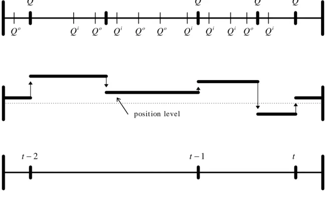
Diagram of data structure

Definitions: Qo is an outgoing interdealer quote (i.e., a quote made) and, if the quote is hit, Ti is the incoming dealer trade. Qi is an incoming interdealer quote (i.e., a quote received) and, if the quote is hit, To is the outgoing trade. Tb is a brokered interdealer trade. Brokered trades do not align vertically with a quote because the data for brokered trades come from the dealer position sheets, and the broker-advertised quotes at the time of the transaction are not recorded. “ “ appears whenever a trade occurs; “│” appears whenever a non-dealt quote occurs. The disjoint segment below the top line represents the dealer's position over the same interval. The time-line at the bottom clarifies the timing relevant to the regression subscripts; namely, periods are defined over incoming transactions.

T

i

Q

o

T

i

Q

o

T

i

Q

o

T

o

Q

i

T

b

Q

o

Q

i

Q

o

Q

i

Q

o

Q

o

Q

i

Q

i

Q

i

Q

o

Q

i

posit ion level

(26)

Figure 2

Diagram of position sheet structure, first fourteen trades on Monday, August 3, 1992

The dealer's position sheets provide the dealer with a running record of his net position and the approximate cost of that position. This dealer fills it in by hand as he trades. Each sheet (page) covers about fifteen transactions. The “Position” column accumulates the individual trades in the “Trade” column. Quantities are in millions of dollars. A positive quantity in the Trade column corresponds to a purchase of dollars. A positive quantity in the Position column corresponds to a net long dollar position. The “Trade Rate” column records the exchange rate for the trade, in deutschemarks per dollar. The “Position Rate” column records the dealer's estimate of the average rate at which he acquired his position. The Position and Position Rate are not calculated after every trade due to time constraints. The “Source” column reports whether the trade is direct over the Reuters Dealing 2000-1 system (r=Reuters) or brokered (b=Broker).

Trade date: 8/3

Value date: 8/5

Position Position rate Trade Trade rate Source Time

1 1.4794 r 8:30 2 1.4797 r 3 1.4796 28 1.4795 r -10 1.4797 r -10 1.4797 b -10 1.4797 r -3 1.4797 b -2 1.4797 0.5 1.4794 r 0.75 1.4790 r 3 1.4791 r 2 1.4791 -10 1.4797 r -8 1.4797 2 1.4799 b -6 1.4797 5 1.4805 b -7 1.4810 r -8 1.4808

(27)

Figure 3

Plot of DM/$ dealer's position I_t (in millions of dollars) from Monday, August 3 to Friday, August 7, 1992.

These positions are constructed from the dealer's position sheets. Short dollar positions corre-spond to long DM positions, and vice versa. The vertical lines designate the four overnight periods through which the dealer did not trade. The relative width of the days is a reflection of the relative trading activity. The two horizontal lines bracketing zero are two standard deviations from the mean long position of two million dollars.

(28)

Figure 4

Plot of DM/$ dealer's total position

I

_t and speculative position

I

$

_ts(in millions of dollars) on Friday from 9AM to 12PM, August 7, 1992.

The total position

I

_t is constructed from the dealer's position sheets. Short dollar positions correspond to long DM positions, and vice versa. The speculative component

I

$

t

s

is estimated as the projection of

I

_t on the information set

Ω

, with

Ω

=

{ }

∆

P

_t,5 , where

∆

P

t,5 is the cumulative

change in the nondealt quotes received by the dealer over the period spanning five incoming trades prior to the incoming trade at t.