Feature Selection Based On Linear Twin Support Vector Machines

Procedia Computer Science 17 ( 2013 ) 1039 – 1046

1877-0509 © 2013 The Authors. Published by Elsevier B.V.

Selection and peer-review under responsibility of the organizers of the 2013 International Conference on Information Technology and Quantitative Management

doi: 10.1016/j.procs.2013.05.132

Information Technology and Quantitative Management, ITQM 2013

Feature Selection Based On Linear Twin Support Vector Machines

a_{Zhijiang College, Zhejiang University of Technology, Hangzhou 310024, P.R.China} b_{College of Science, Zhejiang University of Technology, Hangzhou 310024, P.R.China}

Keywords: Support vector machine, feature selection, twin support vector machine, F-score, SVM-RFE.

1. Introduction

In many machine learning problems, there are hundred even more features, it makes the machine learning algo-rithms consume large calculation. And there are many irrelevant or redundant features among the dataset, it makes the accuracy of the model unsatisfactory. One important way to is the feature selection[1] which delete the irrelevant and redundancy features. After feature selection, the important features are preserved and the redundant features are deleted, which will help to reduce the calculation consumption and increase the accuracy.

Generally, there are two ways to do the feature selection in classification problems. One way is algorithm-independent, such as F-score. F-score is a simple and effective criterion which measures the discrimination of two sets of real numbers [2]. A known deficiency of F-score is that it can not reveal mutual information among features [2]. Another way is algorithm-dependent [3], such as SVM-RFE. In linear SVM, there is a weight vectorw ∈Rn_,

wherenis the number of the features, the larger the|wj|(j=1,· · ·,n) is, the jth feature plays a more important role

in the decision function [4]. Then the weight vectorwcan be used to decide the relevance of each feature [5-6]. One main SVM feature selection algorithm based on this observation is SVM-RFE, the process is (1) Train the classifier; (2) Compute the ranking criterion for all features; (3) Remove the feature with smallest ranking criterion [7]. So we can do the feature selection by using the single weight vector.

∗_{Corresponding author. Tel.:+086-0571-87313679; fax:+086-0571-87313679}

Email address:[email protected](Jun-Yun He) Abstract

By promoting the parallel hyperplanes to non-parallel ones in SVM, twin support vector machines (TWSVM) has been attracted wildly attention. However, the SVM feature selection algorithm (such as SVM-RFE) cannot be used to TWSVM directly. In this paper, we propose two TWSVM feature selection algorithms for classification problems. Firstly, by analyzing the weights in classification, we merge the two weights of the non-parallel hyperplanes in linear TWSVM into one, and propose the sort-TWSVM feature selection by sorting the merged weight; Secondly, inspire by SVM-RFE, we propose the TWSVM-RFE feature selection in a similar way with SVM-RFE by using the merged weight. Preliminary experiments on several benchmark datasets show the feasible and effective of our sort-TWSVM and TWSVM-RFE on feature selection.

© 2013 The Authors. Published by Elsevier B.V.

Selection and peer-review under responsibility of the organizers of the 2013 International Conference on Information Technology and Quantitative Management

Open access under CC BY-NC-ND license.

Recently, Jayadeva et.al proposed the twin support vector machines (TWSVM) [8]. Different from SVM, TWSVM seeks a pair of nonparallel hyperplanes such that each hyperplane is proximal to the data points of one class and far from the data points of the other class [9-11]. It has been shown that in many cases TWSVM is superiority than SVM [12-15]. Different from SVM, in TWSVM [16-23], there are two weight vectors in decision function. Compared with the SVM, the features of the minimum score corresponding tow1may be different fromw2. Thus, we cannot do the feature selection the same as SVM-RFE directly.

In this paper, motivated by SVM-RFE, we propose two TWSVM feature selection algorithms. In TWSVM, the two weight vectors play an important role in decision function, the larger the|wi j|(i = 1,2;j =1,· · ·,n) is, the jth

feature in decision function is more important. Based on the above observation, firstly, we propose a feature selection algorithm based on linear TWSVM, called sort-TWSVM. sort-TWSVM merges the two weight vectors into one vector, then the new weight vector is used to delete the redundant features in a similar way to F-score. sort-TWSVM deletes multiple features disposablely, it is simple with less computational complexity, but the same with the F-score, it does not reveal the mutual information among features. Secondly, we propose another feature selection algorithm based on linear TWSVM, called TWSVM-RFE. TWSVM-RFE also merges the two weight vectors into one, then do feature selection in a similar way with SVM-RFE. Preliminary experiments on several benchmark datasets show the feasible and effective of our sort-TWSVM and TWSVM-RFE on feature selection.

The paper is organized as follows: Section 2 briefly introduces the F-score and SVM-RFE; Section 3 introduces our sort-TWSVM and TWSVM-RFE; Section 4 deals with experimental results; Finally, we offer our conclusions in section 5.

2. F-score and linear SVM for feature selection method

2.1. F-score

F-score is a kind of simple and effective algorithm that measure the difference between two real number sets to feature selection [2]. Given training vector xk(k=1, ...,l), and let the number of positive class and negative class is n₊andn₋respectively. Then thei-th feature’s F-value is given by the following formula:

F(i)≡ (x + i −xi)2+(x−i −xi)2 1 n+−1 n+ k=1 (x+_k,i−x+_i)2₊ 1 n−−1 n− k=1 (x−_k,i−x−_i)2 (1)

wherexi,x+i,x−i is thei-th feature’s average value of all data points, positive points and negative points respectively, x+_k,istands for thei-th feature’s value of thek-th positive points; similarly,x−_k,iis the negative one.

The F-value exactly is the difference between the two points, the larger the value is, the feature is more classifi-cation. The advantage of F-score is that it just uses the guidance of positive and negative labels to get each features’ F-value without any classification algorithm. It is simple and consumes small computational complexity. But this algorithm can not reveal mutual information between features.

2.2. SVM-RFE

For classification, the training dataT ={(x1,y1), ...,(xl,yl)},xi∈Rn,yi={+1,−1},i=1, ...,l. Linear SVM seeks a

hyperplane:

f(x)=wx+b=0 (2)

wherew ∈Rn_{,b ∈R. To measure the empirical risk, the soft margin loss function}l

i=1max(0,1−yi(w·x)+b) is

used. By introducing the regularization term 1/2w2_{and the slack variableξ=(ξ}

1, ξ2, ..., ξl), the primal problem of

SVM can be expressed as min w,b,ξ Φ(w)= 1 2w _w+Cl i=1 ξi (3) s.t. yi(wxi+b)≥1−ξi, ξi≥0 i=1, ...,l (4)

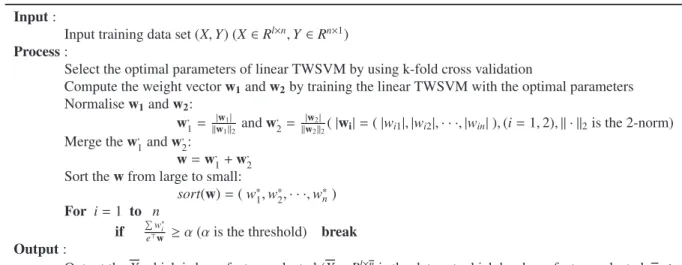
Table 1: Algorithm 1. sort-TWSVM

Input:

Input training data set (X,Y) (X∈Rl×n_{,Y ∈R}n×1₎ Process:

Select the optimal parameters of linear TWSVM by using k-fold cross validation

Compute the weight vectorw1andw2by training the linear TWSVM with the optimal parameters

Normalisew1andw2: w,₁= |w1| w12 andw , 2= |w2| w22(|wi|=(|wi1|,|wi2|,· · ·,|win|),(i=1,2), · 2is the 2-norm)

Merge thew,₁andw,₂:

w=w,₁+w,₂

Sort thewfrom large to small:

sort(w)=(w∗₁,w∗₂,· · ·,w∗n)

For i=1 to n

if

w∗_i

ew ≥α(αis the threshold) break Output:

Output theXwhich is been feature selected (X∈Rl×n_{is the data set which has been feature selected,n≤n)}

whereCis the punish parameter. Solving this optimization problem, we can get the weight vectorwand the constant

b, the decision function follows:

f(x)=sgn(wx+b) (5)

Every component of the weight vector is the weight value of the corresponding feature. The larger|wj|is, the j-th

feature plays a more important role in the decision function [4]. The process of SVM-RFE is (1) Train the classifier; (2) Compute the ranking criterion for all features; (3) Remove the feature with smallest ranking criterion [7].

Experimental results show that the SVM-RFE can output the results steadily. Though SVM-RFE consumes large calculation because it delete one feature at one time, it reveals the mutual information among features.

3. Feature selection based on linear TWSVM

Suppose that all of the input in class+1 are denotedA∈Rl1×n_{. Similarly, the matrixB}∈_Rl2×n_{represents the input}

of class−1. Different from SVM, TWSVM seeks a pair of nonparallel hyperplanes[8]:

f1(x)=w1x+b1 and f2(x)=w2x+b2, (6)

such that each hyperplane is proximal to the data points of one class and far from the data points of the other class, wherew1,w2∈Rn,b1,b2∈R. The optimal problems of TWSVM [9] expressed as

min w1,b1,ξ,ξ∗ 1 2c3(w1 2_+b2 1)+ 1 2ξ ∗_ξ∗_+c 1e2ξ (7) s.t. Aw1+e1b1=ξ∗ (8) −(Bw1+e2b1)+ξ≥e2, ξ≥0 (9) and min w2,b2,η,η∗ 1 2c4(w2 2_+b2 2)+ 1 2η ∗_η∗_+c 2e1η (10) s.t. Bw2+e2b2=η∗ (11) (Aw2+e1b2)+η≥e1, η≥0 (12)

Table 2: Algorithm 2. TWSVM-RFE

Input:

Input training data set (X,Y)

Process:

Repeat

Select the optimal parameters of linear TWSVM by using k-fold cross validation

Compute the weight vectorw1andw2by training the linear TWSVM with the potimal parameters

Normalisew1andw2: w,₁= |w1| w12 andw , 2= |w2|

w22(|wi|=(|wi1|,|wi2|,· · ·,|win|),(i=1,2), · 2is the 2-norm)

Merge thew,₁andw,₂:

w=w,₁+w,₂

Sort thewfrom small to large:

sort(w)=(w∗1,w∗2,· · ·,w∗n)

if w∗1

ew≤β(β is the threshold)

Delete the feature which the w∗₁ corresponding to and update the inputX

else break Output:

Output theXwhich is feature selected (X∈Rl×n_{is the data set which has been feature selected,n≤n)}

wherec1,c2,c3andc4are positive parameters,ξ,ξ∗,ηandη∗are slack variables.

By solving the above two problems, we can get two weight vectorsw1,w2and two constantsb1,b2. From this we

construct two hyperplanesf1(x)=w₁x+b1andf2(x)=w₂x+b2. The decision function of the TWSVM is

Class i=arg min

k=1,2

|w_kx+bk|

wk

(13) In the decision function,|w_kx+bk|=|wk1·xi1+wk2·xi2· · ·+wkn·xin+bk|(k=1,2;i=1,· · ·,l). The reason why we

can not use SVM-RFE[7] directly is that,w1jandw2j(j=1,· · ·,n) may be not large or small at the same time, we can

not use only one of them to do feature selection. But every component of the weight vector is the weight value of each features. The larger|wk j|(k=1,2;j=1,· · ·,n) is, the jth feature plays a more important role in the decision function

[4,8]. Based on the above observation, we propose the sort-TWSVM algorithm in Table.1. sort-TWSVM mergers the two weight vectors into one, the new weight vector is used to delete the redundant features in a similar way to F-score. This algorithm is convergence and play the role of feature selection. However, we can not control the number of the features selected in sort-TWSVM. According to SVM-RFE [7], we strictly extend the sort-TWSVM to another feature selection algorithm, called TWSVM-RFE, and we present the second algorithm in Table 2. Our TWSVM-RFE cuts out the feature with minimum score similar to SVM-RFE. Compare to sort-TWSVM, this algorithm consumes more computational complexity. But this algorithm reveals the mutual information among features.

4. Experiments

In this section, some experiments are made to demonstrate the performance of our feature selection algorithms. All algorithms are implemented by using MATLAB 7.0 [19] on a PC with an Intel Core i3-2350M processor (2.3 GHz) with 4 GB RAM. Classification accuracy of each algorithm is measured by the standard tenfold cross-validation methodology [20]. And we pick up the optimal parametersc1,c2,c3andc4of each data in the range 2−8to 27. Once

the parameters are selected, the tuning set is returned to learn the final classifier.

In order to compare the behavior of our two feature selection algorithms, we choose the datasets which are from the UCI [21] machine learning repository. The results of numerical experiments are summarized in Table 3. Here,

Table 3: The accuracy (%) on UCI data sets for linear classifiers

Datasets TWSVM F-score+TWSVM sort-TWSVM TWSVM-RFE

Accuracy(%) Accuracy(%) Accuracy(%) Accuracy(%)

Feature Feature Feature Feature

(c1=c2)/(c3=c4) (c1=c2)/(c3=c4) (c1=c2)/(c3=c4) (c1=c2)/(c3=c4) Australian 86.78±1.90 75.22±3.50 86.62±2.29 86.38±3.69 (690×14) 14 4 11 5 4/128 2/0.25 0.125/0.125 0.0156/1 CMC 77.39±4.61 77.93±1.37 77.38±4.20 77.32±3.52 (1473×9) 9 6 7 6 0.5/0.0039 0.5/0.0039 0.5/64 0.5/16 Echocardiogram 90.99±6.21 89.39±2.52 90.00±1.10 90.99±2.33 (131×10) 10 9 9 7 8/128 0.25/0.25 0.0039/2 0.0625/0.5 German 76.63±3.16 69.96±3.21 76.13±4.02 76.80±2.55 (1000×20) 20 9 15 11 0.5/0.0156 1/128 0.5/0.0078 0.5/32 Haberman 74.67±1.15 26.47±0 74.62±1.56 74.66±1.25 (306×3) 3 1 3 3 0.0039/8 0.0039/0.0039 0.0039/8 0.0039/8 Monks3 66.62±2.83 66.67±1.37 67.29±1.95 66.67±1.37 (432×6) 6 1 4 1 0.0078/0.0078 0.0039/0.0039 0.0625/1 0.0039/0.0039 Sonar 78.63±5.54 75.34±2.69 79.62±1.09 80.77±1.22 (208×60) 60 37 49 8 64/256 0.25/0.0078 64/0.0313 4/0.0156 hepatitis 81.29±7.03 83.74±3.51 83.10±1.28 88.52±3.03 (155×19) 19 9 15 8 32/0.0078 0.0078/8 2/0.0625 0.125/0.25 WPBC 84.14±3.33 75.61±3.99 82.93±2.54 77.93±1.53 (198×34) 34 24 26 11 0.0156/0.0039 0.5/8 2/0.0313 0.25/0.125

the classification accuracy, feature number and the optimal parameters (c1 =c2andc3 =c4) are listed, and the best accuracy is shown by bold figures. From the Table 3, it is easy to see that the our two feature selection algorithms delete the redundant features and obtain better classification results, for example, for Sonar data, the number of the selected features by TWSVM-RFE is 8, while the accuracy is 80.77%, while TWSVM obtains 78.63% with 60 features. That is to say, both sort-TWSVM and TWSVM-RFE can do feature selection well, while sort-TWSVM with a fast speed and TWSVM-RFE with a better feature selection capability.

In order to study the behavior of our two feature selection algorithms further, the two-dimensional scatter plots were used in [10, 18]. The corresponding scatter plots are shown in Fig. 1 for two UCI datasets (hepatitis and Sonar datasets) with about 20 percent of data points. The plots are obtained by plotting points with coordinates (d_i+,d_i−), whered±_i are the respective distances of a test point xifrom the two projections. From Fig. 1, generally speaking,

the distances between the most test points and the corresponding projection is small for both TWSVM-RFE and our TWSVM, but only for our TWSVM-RFE the distances between the most test points and the opposite projection are rather large while for TWSVM are also small.

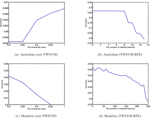
At last, we analysis the relationship between the accuracy and the thresholdαin sort-TWSVM and TWSVM-RFE. Fig. 2 shows the relationship between the accuracy and the thresholdαon the Australian and Madelon data sets. From the Fig. 2 (a) and (b), we obtain that for Australian data, the results of two feature selection algorithms are similar in

0 0.5 1 1.5 2 2.5 0 0.5 1 1.5 2 2.5 d1 d2 (a) hepatitis (TWSVM) 0 1 2 3 4 0 0.5 1 1.5 2 2.5 3 3.5 4 d1 d2 (b) hepatitis (TWSVM-RFE) 0 0.2 0.4 0.6 0.8 1 1.2 1.4 0 0.2 0.4 0.6 0.8 1 1.2 1.4 d1 d2 (c) Sonar (TWSVM) 0 0.2 0.4 0.6 0.8 1 1.2 1.4 0 0.2 0.4 0.6 0.8 1 1.2 1.4 d1 d2 (d) Sonar (TWSVM-RFE)

Fig. 1: The experimental results on hepatitis(155×19) and Sonar(208×60) datasets. Figure(a) and (c) are the results of TWSVM, Figure(b) and (d) are the results of TWSVM-RFE, where the abscissa axis stands for the distance between a point and hyperplanef1, we denote it asd1. Similarly,

the ordinate axis stands for the distance between a point and hyperplanef2, we denote it asd2. The diagonal in each figure means the points which

d1=d2. We mark the points of class -1 as red “x”, and mark the points of class+1 as blue “o”. Thus, the blue points which above the diagonal is

0.8 0.85 0.9 0.95 1 0.856 0.858 0.86 0.862 0.864 0.866 0.868 0.87

The threshold value

Accuracy

(a) Australian (sort-TWSVM)

0 2 4 6 8 10 12 14 0.55 0.6 0.65 0.7 0.75 0.8 0.85 0.9 0.95

The number of deleted features

Accuracy (b) Australian (TWSVM-RFE) 0.8 0.85 0.9 0.95 1 0.6 0.61 0.62 0.63 0.64 0.65 0.66

The threshold value

Accuracy (c) Madelon (sort-TWSVM) 0 50 100 150 200 250 0.59 0.6 0.61 0.62 0.63 0.64 0.65 0.66

The number of deleted features

Accuracy

(d) Madelon (TWSVM-RFE)

Fig. 2: The experimental results on the Australian(690×14) and Madelon(2000×500) datasets. Figure(a) and (c) show the relationship between accuracy and the thresholdαby sort-TWSVM. Figure(b) and (d) show the relationship between accuracy and the number of deleted features by TWSVM-RFE.

this dataset, where most features play a positive rule in classification. From the Fig. 2 (c) and (d), we obtain that for Madelon data, there are a lot of redundancy features, we can see that the larger the number of deleted features is, the less the accuracy is. That is to say, by using these features will reduce classification accuracy, and both sort-TWSVM and TWSVM-RFE can exploit this characteristic.

5. Conclusion

In this paper, we have proposed two feature selection algorithms (sort-TWSVM and TWSVM-RFE). By merging the two weight vectors into ones, sort-TWSVM deletes the smaller weight components disposable, while TWSVM-RFE just deletes the smallest weight component at a time, and do feature selection in a similar way with SVM-TWSVM-RFE by using the merged weight. Experimental results on several benchmark datasets show the feasible and effective of our sort-TWSVM and TWSVM-RFE on feature selection. In the future, we will study the difference between the two feature selection algorithms, such as whether the deleted features are same to a dataset or how many features are same. Then, we will pick up the optimal thresholdsαandβto control the number of features and to get the optimal accuracy. At last, we can research our two feature selection algorithms by usingL1-norm TWSVM.

Acknowledgments

This work is supported by the National Natural Science Foundation of China (No.11201426, No. 10971223 and No. 11071252), the Zhejiang Provincial Natural Science Foundation of China (No.LQ12A01020) and the Science and Technology Foundation of Department of Education of Zhejiang Province (No. Y201225256 and No.Y201225179).

References

[1] K.Q. Shen, C.J. Ong, X.P. Li, Einar P.V. and Wilder-Smith, Feature selection via sensitivity analysis of SVM probabilistic outputs. Machine Learning, 2008, 70:1-20.

[2] Y.W. Chang, C.J. Lin, Combining SVMs with various feature selection strategies. Studies in Fuzziness and Soft Computing, 2006, 207:315-324

[3] A. Blum and P. Langley, Selection of relevant features and examples in machine learning. Artificial intelligence, 1997, 97:245-271. [4] Y.W. Chang, C.J. Lin, Feature Ranking Using Linear SVM. JMLR Workshop and Conference Proceedings, 2008, 3:53-64.

[5] Yitian Xu, Ping Zhong, Laisheng Wang, Support vector machine-based embedded approach feature selection algorithm, Journal of Informa-tion and ComputaInforma-tional Science, 7 (5) (2010), 1155-1163

[6] C.H. Zhang, Y.H. Shao, J.Y. Tan, N.Y. Deng, Mixed-norm linear support vector machine, Neural Computing and Applications, 2012, 10.1007/s00521-012-1166-0

[7] Isabelle Guyon, Jason Weston, Stephen Barnhill and Vladimir Vapnik, Gene selection for cancer classification using support vector machines. Machine Learning, 2002, 46:389-422.

[8] Jayadeva, R.Khemchandani, Suresh Chandra, Twin support vector machines for pattern classification, IEEE transaction on patterns analysis and machine intelligence, 2007, 29:905-910.

[9] Y.H. Shao, C.H. Zhang, X.B. Wang and N.Y. Deng, Improvements on twin support vector machines. IEEE transactions on neural networks, 2011, 22:962-968.

[10] Y.H. Shao, Z. Wang, W.J. Chen, N.Y. Deng, A regularization for the projection twin support vector machine. Knowledge-Based Systems, 2013, 37:203-210

[11] Y.H. Shao, N.Y. Deng, A coordinate descent margin based-twin support vector machine for classification. Neural Networks, 2012, 25:114-121.

[12] Y.H. Shao, N.Y. Deng, W.J. Chen, Z. Wang, Improved generalized eigenvalue proximal support vector machine. IEEE Signal Processing Letters, 2013, 20(3):213-216.

[13] Z. Qi, Y. Tian, S. Yong, Robust twin support vector machine for pattern classification. Pattern Recognition, 2012, 46(1):305-316.

[14] Y. Tian, Y. Shi, X. Liu, Recent advances on support vector machines research, Technological and Economic Development of Economy, 2012, 18(1):5-33.

[15] Y.H. Shao, C.H. Zhang, Z.M. Yang, L. Jing, N.Y. Deng, Anε-twin support vector machine for regression. Neural Comput Applic, 2012, doi: 10.1007/s00521-012-0924-3

[16] Qi Z, Tian Y, Shi Y, Laplacian twin support vector machine for semi-supervised classiffication. Neural Networks, 2012, 35:46-53.

[17] Y.H. Shao, N.Y. Deng, Z.M. Yang, W.J. Chen, Z. Wang, Probabilistic outputs for twin support vector machines. Knowledge Based Systems, 2012, 33:145-151

[18] Y.H. Shao, N.Y. Deng, Z.M. Yang, Least squares recursive projection twin support vector machine for classification. Pattern Recognition, 2012, 45(6): 2299-2307.

[19] MathWorks. 2007. [Online]. Available: http://www.mathworks.com

[20] R. O. Duda, P. E. Hart, and D. G. Stork, Pattern Classification, 2nd ed. New York: Wiley, 2001.

[21] C. L. Blake and C. J. Merz. UCI Repository for Machine Learning Databases. Dept. Inf. Comput. Sci., Univ. California, Irvine[Online]. 1998. Available: http://www.ics.uci.edu/∼mlearn/MLRepository.html

[22] Z. Qi, Y. Tian, S. Yong, Twin support vector machine with Universum data, Neural Networks, 2012, 36C:112-119

[23] Z. Qi, Y. Tian, and Y. Shi, Structural Twin Support Vector Machine for Classification, Knowledge-Based Systems, 2013, DOI: 10.1016/j.knosys.2013.01.008