Cluster Analysis
Keywords Agglomerative and divisive clustering Chebychev distance
City-block distance Clustering variables Dendrogram Distance matrix
Euclidean distance Hierarchical and partitioning methods Icicle diagram
k-meansMatching coefficientsProfiling clustersTwo-step clustering
Introduction
Grouping similar customers and products is a fundamental marketing activity. It is used, prominently, in market segmentation. As companies cannot connect with all their customers, they have to divide markets into groups of consumers, customers, or clients (called segments) with similar needs and wants. Firms can then target each of these segments by positioning themselves in a unique segment (such as Ferrari in the high-end sports car market). While market researchers often form
Learning Objectives
After reading this chapter you should understand: – The basic concepts of cluster analysis. – How basic cluster algorithms work.
– How to compute simple clustering results manually. – The different types of clustering procedures. – The SPSS clustering outputs.
Are there any market segments where Web-enabled mobile telephony is taking off in different ways? To answer this question, Okazaki (2006) applies a two-step cluster analysis by identifying segments of Internet adopters in Japan. The findings suggest that there are four clusters exhibiting distinct attitudes towards Web-enabled mobile telephony adoption. Interestingly, freelance, and highly educated professionals had the most negative perception of mobile Internet adoption, whereas clerical office workers had the most positive perception. Furthermore, housewives and company executives also exhibited a positive attitude toward mobile Internet usage. Marketing managers can now use these results to better target specific customer segments via mobile Internet services.
E. Mooi and M. Sarstedt,A Concise Guide to Market Research,
DOI 10.1007/978-3-642-12541-6_9,#Springer-Verlag Berlin Heidelberg 2011
market segments based on practical grounds, industry practice and wisdom, cluster analysis allows segments to be formed that are based on data that are less dependent on subjectivity.
The segmentation of customers is a standard application of cluster analysis, but it can also be used in different, sometimes rather exotic, contexts such as evaluating
typical supermarket shopping paths (Larson et al. 2005) or deriving employers’
branding strategies (Moroko and Uncles2009).
Understanding Cluster Analysis
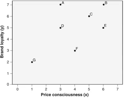
Cluster analysis is a convenient method for identifying homogenous groups of objects called clusters. Objects (or cases, observations) in a specific cluster share many characteristics, but are very dissimilar to objects not belonging to that cluster. Let’s try to gain a basic understanding of the cluster analysis procedure by looking at a simple example. Imagine that you are interested in segmenting your customer base in order to better target them through, for example, pricing strategies. The first step is to decide on the characteristics that you will use to segment your customers. In other words, you have to decide which clustering variables will be included in the analysis. For example, you may want to segment a market based on
customers’ price consciousness (x) and brand loyalty (y). These two variables can
be measured on a 7-point scale with higher values denoting a higher degree of price consciousness and brand loyalty. The values of seven respondents are shown in
Table9.1and the scatter plot in Fig.9.1.
The objective of cluster analysis is to identify groups of objects (in this case, customers) that are very similar with regard to their price consciousness and brand loyalty and assign them into clusters. After having decided on the clustering variables (brand loyalty and price consciousness), we need to decide on the clustering procedure to form our groups of objects. This step is crucial for the analysis, as different procedures require different decisions prior to analysis. There is an abundance of different approaches and little guidance on which one to use in practice. We are going to discuss the most popular approaches in market research,
as they can be easily computed using SPSS. These approaches are:hierarchical
methods,partitioning methods(more precisely,k-means), andtwo-step clustering, which is largely a combination of the first two methods. Each of these procedures follows a different approach to grouping the most similar objects into a cluster and to determining each object’s cluster membership. In other words, whereas an object in a certain cluster should be as similar as possible to all the other objects in the
Table 9.1 Data
Customer A B C D E F G
x 3 6 5 3 6 4 1
same cluster, it should likewise be as distinct as possible from objects in different clusters.
But how do we measure similarity? Some approaches – most notably hierarchi-cal methods – require us to specify how similar or different objects are in order to identify different clusters. Most software packages calculate a measure of (dis)similarity by estimating the distance between pairs of objects. Objects with smaller distances between one another are more similar, whereas objects with larger distances are more dissimilar.
An important problem in the application of cluster analysis is the decision regarding how many clusters should be derived from the data. This question is explored in the next step of the analysis. Sometimes, however, we already know the number of segments that have to be derived from the data. For example, if we were asked to ascertain what characteristics distinguish frequent shoppers from infre-quent ones, we need to find two different clusters. However, we do not usually know the exact number of clusters and then we face a trade-off. On the one hand, you want as few clusters as possible to make them easy to understand and action-able. On the other hand, having many clusters allows you to identify more segments and more subtle differences between segments. In an extreme case, you can address each individual separately (called one-to-one marketing) to meet consumers’ vary-ing needs in the best possible way. Examples of such a micro-marketvary-ing strategy
are Puma’s Mongolian Shoe BBQ (www.mongolianshoebbq.puma.com) and Nike
ID (http://nikeid.nike.com), in which customers can fully customize a pair of shoes in a hands-on, tactile, and interactive shoe-making experience. On the other hand, the costs associated with such a strategy may be prohibitively high in many
B A E C F Brand loyalty (y ) G Price consciousness (x) D 7 6 5 4 3 2 1 0 0 1 2 3 4 5 6 7
business contexts. Thus, we have to ensure that the segments are large enough to make the targeted marketing programs profitable. Consequently, we have to cope with a certain degree of within-cluster heterogeneity, which makes targeted marketing programs less effective.
In the final step, we need to interpret the solution by defining and labeling the obtained clusters. This can be done by examining the clustering variables’ mean values or by identifying explanatory variables to profile the clusters. Ultimately, managers should be able to identify customers in each segment on the basis of easily measurable variables. This final step also requires us to assess the clustering
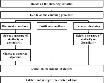
solution’s stability and validity. Figure9.2illustrates the steps associated with a
cluster analysis; we will discuss these in more detail in the following sections.
Conducting a Cluster Analysis
Decide on the Clustering Variables
At the beginning of the clustering process, we have to select appropriate variables for clustering. Even though this choice is of utmost importance, it is rarely treated as such and, instead, a mixture of intuition and data availability guide most analyses in marketing practice. However, faulty assumptions may lead to improper market
Decide on the clustering variables
Decide on the clustering procedure
Hierarchical methods Partitioning methods Two-step clustering
Select a measure of similarity or dissimilarity Select a measure of similarity or dissimilarity Choose a clustering algorithm
Decide on the number of clusters
Validate and interpret the cluster solution
segments and, consequently, to deficient marketing strategies. Thus, great care should be taken when selecting the clustering variables.
There are several types of clustering variables and these can be classified into
general(independent of products, services or circumstances) andspecific(related to both the customer and the product, service and/or particular circumstance),
on the one hand, and observable (i.e., measured directly) and unobservable
(i.e., inferred) on the other. Table 9.2 provides several types and examples of
clustering variables.
The types of variables used for cluster analysis provide different segments and, thereby, influence segment-targeting strategies. Over the last decades, attention has shifted from more traditional general clustering variables towards product-specific unobservable variables. The latter generally provide better guidance for decisions on marketing instruments’ effective specification. It is generally acknowledged that segments identified by means of specific unobservable variables are usually more homogenous and their consumers respond consistently to marketing actions (see
Wedel and Kamakura 2000). However, consumers in these segments are also
frequently hard to identify from variables that are easily measured, such as demo-graphics. Conversely, segments determined by means of generally observable variables usually stand out due to their identifiability but often lack a unique
response structure.1 Consequently, researchers often combine different variables
(e.g., multiple lifestyle characteristics combined with demographic variables), benefiting from each ones strengths.
In some cases, the choice of clustering variables is apparent from the nature of the task at hand. For example, a managerial problem regarding corporate communi-cations will have a fairly well defined set of clustering variables, including con-tenders such as awareness, attitudes, perceptions, and media habits. However, this is not always the case and researchers have to choose from a set of candidate variables.
Whichever clustering variables are chosen, it is important to select those that provide a clear-cut differentiation between the segments regarding a specific
managerial objective.2More precisely, criterion validity is of special interest; that
is, the extent to which the “independent” clustering variables are associated with
Table 9.2 Types and examples of clustering variables
General Specific
Observable (directly measurable)
Cultural, geographic, demographic, socio-economic
User status, usage frequency, store and brand loyalty Unobservable
(inferred)
Psychographics, values, personality, lifestyle
Benefits, perceptions, attitudes, intentions, preferences Adapted from Wedel and Kamakura (2000)
1See Wedel and Kamakura (2000).
2Tonks (2009) provides a discussion of segment design and the choice of clustering variables in consumer markets.
one or more “dependent” variables not included in the analysis. Given this relation-ship, there should be significant differences between the “dependent” variable(s) across the clusters. These associations may or may not be causal, but it is essential that the clustering variables distinguish the “dependent” variable(s) significantly. Criterion variables usually relate to some aspect of behavior, such as purchase intention or usage frequency.
Generally, you should avoid using an abundance of clustering variables, as this increases the odds that the variables are no longer dissimilar. If there is a high degree of collinearity between the variables, they are not sufficiently unique to identify distinct market segments. If highly correlated variables are used for cluster analysis, specific aspects covered by these variables will be overrepresented in the clustering solution. In this regard, absolute correlations above 0.90 are always
problematic. For example, if we were to add another variable calledbrand
pre-ferenceto our analysis, it would virtually cover the same aspect asbrand loyalty. Thus, the concept of being attached to a brand would be overrepresented in the analysis because the clustering procedure does not differentiate between the clus-tering variables in a conceptual sense. Researchers frequently handle this issue by applying cluster analysis to the observations’ factor scores derived from a
previously carried out factor analysis. However, according to Dolnicar and Gr€un
(2009), this factor-cluster segmentation approach can lead to several problems:
1. The data are pre-processed and the clusters are identified on the basis of trans-formed values, not on the original information, which leads to different results. 2. In factor analysis, the factor solution does not explain a certain amount of
variance; thus, information is discarded before segments have been identified or constructed.
3. Eliminating variables with low loadings on all the extracted factors means that, potentially, the most important pieces of information for the identification of niche segments are discarded, making it impossible to ever identify such groups. 4. The interpretations of clusters based on the original variables become
question-able given that the segments have been constructed using factor scores. Several studies have shown that the factor-cluster segmentation significantly
reduces the success of segment recovery.3Consequently, you should rather reduce
the number of items in the questionnaire’s pre-testing phase, retaining a reasonable number of relevant, non-redundant questions that you believe differentiate the segments well. However, if you have your doubts about the data structure, factor-clustering segmentation may still be a better option than discarding items that may conceptually be necessary.
Furthermore, we should keep the sample size in mind. First and foremost, this relates to issues of managerial relevance as segments’ sizes need to be substan-tial to ensure that targeted marketing programs are profitable. From a statistical perspective, every additional variable requires an over-proportional increase in
observations to ensure valid results. Unfortunately, there is no generally accepted rule of thumb regarding minimum sample sizes or the relationship between the objects and the number of clustering variables used.
In a related methodological context, Formann (1984) recommends a sample size
of at least2m, wheremequals the number of clustering variables. This can only
provide rough guidance; nevertheless, we should pay attention to the relationship between the objects and clustering variables. It does not, for example, appear logical to cluster ten objects using ten variables. Keep in mind that no matter how many variables are used and no matter how small the sample size, cluster analysis will always render a result!
Ultimately, the choice of clustering variables always depends on contextual influences such as data availability or resources to acquire additional data. Market-ing researchers often overlook the fact that the choice of clusterMarket-ing variables is closely connected to data quality. Only those variables that ensure that high quality data can be used should be included in the analysis. This is very important if a segmentation solution has to be managerially useful. Furthermore, data are of high quality if the questions asked have a strong theoretical basis, are not contaminated by respondent fatigue or response styles, are recent, and thus reflect the current
market situation (Dolnicar and Lazarevski2009). Lastly, the requirements of other
managerial functions within the organization often play a major role. Sales and distribution may as well have a major influence on the design of market segments. Consequently, we have to be aware that subjectivity and common sense agreement will (and should) always impact the choice of clustering variables.
Decide on the Clustering Procedure
By choosing a specific clustering procedure, we determine how clusters are to be formed. This always involves optimizing some kind of criterion, such as minimiz-ing the within-cluster variance (i.e., the clusterminimiz-ing variables’ overall variance of objects in a specific cluster), or maximizing the distance between the objects or clusters. The procedure could also address the question of how to determine the (dis)similarity between objects in a newly formed cluster and the remaining objects in the dataset.
There are many different clustering procedures and also many ways of classify-ing these (e.g., overlappclassify-ing versus non-overlappclassify-ing, unimodal versus multimodal,
exhaustive versus non-exhaustive).4A practical distinction is the differentiation
betweenhierarchicalandpartitioning methods(most notably thek-meansprocedure),
which we are going to discuss in the next sections. We also introduce two-step
clustering, which combines the principles of hierarchical and partitioning methods and which has recently gained increasing attention from market research practice.
4See Wedel and Kamakura (2000), Dolnicar (2003), and Kaufman and Rousseeuw (2005) for a review of clustering techniques.
Hierarchical Methods
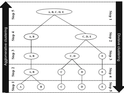
Hierarchical clustering procedures are characterized by the tree-like structure established in the course of the analysis. Most hierarchical techniques fall into a
category called agglomerative clustering. In this category, clusters are
consecu-tively formed from objects. Initially, this type of procedure starts with each object representing an individual cluster. These clusters are then sequentially merged according to their similarity. First, the two most similar clusters (i.e., those with the smallest distance between them) are merged to form a new cluster at the bottom of the hierarchy. In the next step, another pair of clusters is merged and linked to a higher level of the hierarchy, and so on. This allows a hierarchy of clusters to be
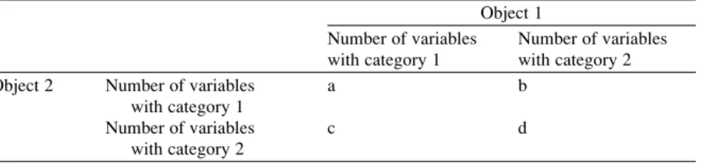
established from the bottom up. In Fig.9.3(left-hand side), we show how
agglome-rative clustering assigns additional objects to clusters as the cluster size increases.
A cluster hierarchy can also be generated top-down. In thisdivisive clustering,
all objects are initially merged into a single cluster, which is then gradually split up.
Figure9.3illustrates this concept (right-hand side). As we can see, in both
agglom-erative and divisive clustering, a cluster on a higher level of the hierarchy always encompasses all clusters from a lower level. This means that if an object is assigned to a certain cluster, there is no possibility of reassigning this object to another cluster. This is an important distinction between these types of clustering and partitioning methods such as k-means, which we will explore in the next section.
Divisive procedures are quite rarely used in market research. We therefore concentrate on the agglomerative clustering procedures. There are various types
A, B, C, D, E Step 5 Step 1 C, D, E A, B Step 2 C, D Ag glomerative clustering Divisive clustering E A, B Step 3 Step 4 A, B C D E Step 2 Step 4 Step 3 A B C D E Step 1 Step 5
of agglomerative procedures. However, before we discuss these, we need to define how similarities or dissimilarities are measured between pairs of objects.
Select a Measure of Similarity or Dissimilarity
There are various measures to express (dis)similarity between pairs of objects. A straightforward way to assess two objects’ proximity is by drawing a straight line
between them. For example, when we look at the scatter plot in Fig.9.1, we can
easily see that the length of the line connecting observations B and C is much shorter than the line connecting B and G. This type of distance is also referred to as
Euclidean distance(or straight-line distance) and is the most commonly used type
when it comes to analyzing ratio or interval-scaled data.5In our example, we have
ordinal data, but market researchers usually treat ordinal data as metric data to calculate distance metrics by assuming that the scale steps are equidistant (very
much like in factor analysis, which we discussed in Chap.8). To use a hierarchical
clustering procedure, we need to express these distances mathematically. By taking
the data in Table 9.1 into consideration, we can easily compute the Euclidean
distance between customer B and customer C (generally referred to as d(B,C))
with regard to the two variablesxandyby using the following formula:
dEuclideanðB;CÞ ¼ ffiffiffiffiffiffiffiffiffiffiffiffiffiffiffiffiffiffiffiffiffiffiffiffiffiffiffiffiffiffiffiffiffiffiffiffiffiffiffiffiffiffiffiffiffiffiffiffi xBxC ð Þ2 þðyByCÞ2 q
The Euclidean distance is the square root of the sum of the squared differences in
the variables’ values. Using the data from Table9.1, we obtain the following:
dEuclideanðB;CÞ ¼ ffiffiffiffiffiffiffiffiffiffiffiffiffiffiffiffiffiffiffiffiffiffiffiffiffiffiffiffiffiffiffiffiffiffiffiffiffiffiffi 65 ð Þ2 þ 76 ð Þ2 q ¼pffiffiffi2¼1:414
This distance corresponds to the length of the line that connects objects B and C. In this case, we only used two variables but we can easily add more under the root sign in the formula. However, each additional variable will add a dimension to our research problem (e.g., with six clustering variables, we have to deal with six dimensions), making it impossible to represent the solution graphically. Similarly, we can compute the distance between customer B and G, which yields the following:
dEuclideanðB;GÞ ¼ ffiffiffiffiffiffiffiffiffiffiffiffiffiffiffiffiffiffiffiffiffiffiffiffiffiffiffiffiffiffiffiffiffiffiffiffiffiffiffi 61 ð Þ2þ 72 ð Þ2 q ¼pffiffiffiffiffi50¼7:071
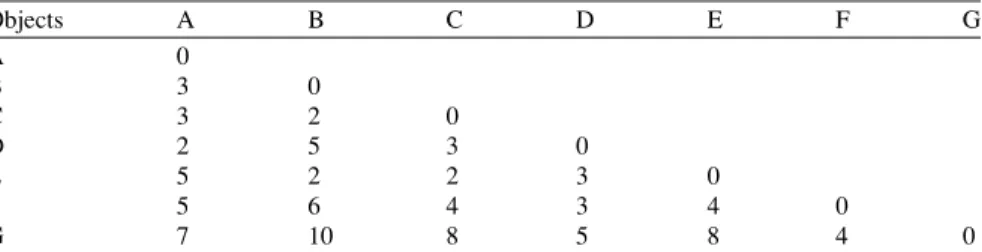
Likewise, we can compute the distance between all other pairs of objects. All
these distances are usually expressed by means of adistance matrix. In this distance
matrix, the non-diagonal elements express the distances between pairs of objects
and zeros on the diagonal (the distance from each object to itself is, of course, 0). In
our example, the distance matrix is an 8 8 table with the lines and rows
representing the objects (i.e., customers) under consideration (see Table9.3). As
the distance between objects B and C (in this case 1.414 units) is the same as between C and B, the distance matrix is symmetrical. Furthermore, since the distance between an object and itself is zero, one need only look at either the lower or upper non-diagonal elements.
There are also alternative distance measures: Thecity-block distanceuses the
sum of the variables’ absolute differences. This is often called the Manhattan metric as it is akin to the walking distance between two points in a city like New York’s Manhattan district, where the distance equals the number of blocks in the directions North-South and East-West. Using the city-block distance to compute the distance between customers B and C (or C and B) yields the following:
dCityblockðB;CÞ ¼jxBxCj þjyByCj ¼j65j þj76j ¼2
The resulting distance matrix is in Table9.4.
Lastly, when working with metric (or ordinal) data, researchers frequently use theChebychev distance, which is the maximum of the absolute difference in the clustering variables’ values. In respect of customers B and C, this result is:
dChebychecðB;CÞ ¼maxðjxBxCj;jyByCjÞ ¼max 6ðj 5j;j76jÞ ¼1
Figure 9.4 illustrates the interrelation between these three distance measures
regarding two objects, C and G, from our example.
Table 9.4 City-block distance matrix
Objects A B C D E F G A 0 B 3 0 C 3 2 0 D 2 5 3 0 E 5 2 2 3 0 F 5 6 4 3 4 0 G 7 10 8 5 8 4 0
Table 9.3 Euclidean distance matrix
Objects A B C D E F G A 0 B 3 0 C 2.236 1.414 0 D 2 3.606 2.236 0 E 3.606 2 1.414 3 0 F 4.123 4.472 3.162 2.236 2.828 0 G 5.385 7.071 5.657 3.606 5.831 3.162 0
There are other distance measures such as the Angular, Canberra or Mahalanobis distance. In many situations, the latter is desirable as it compensates for collinearity between the clustering variables. However, it is (unfortunately) not menu-accessible in SPSS.
In many analysis tasks, the variables under consideration are measured on different scales or levels. This would be the case if we extended our set of clustering variables by adding another ordinal variable representing the customers’ income measured by means of, for example, 15 categories. Since the absolute variation of the income variable would be much greater than the variation of the remaining
two variables (remember, thatxandyare measured on 7-point scales), this would
clearly distort our analysis results. We can resolve this problem by standardizing the data prior to the analysis.
Different standardization methods are available, such as the simple z standardi-zation, which rescales each variable to have a mean of 0 and a standard deviation of
1 (see Chap.5). In most situations, however, standardization by range (e.g., to a
range of 0 to 1 or1 to 1) performs better.6We recommend standardizing the data
in general, even though this procedure can reduce or inflate the variables’ influence on the clustering solution.
C
Euclidean distance City-block distance
Brand loyalty (y)
G
Chebychev distance
Price consciousness (x) Fig. 9.4 Distance measures
Another way of (implicitly) standardizing the data is by using the correlation between the objects instead of distance measures. For example, suppose a respon-dent rated price consciousness 2 and brand loyalty 3. Now suppose a second respondent indicated 5 and 6, whereas a third rated these variables 3 and 3. Eucli-dean, city-block, and Chebychev distances would indicate that the first respondent is more similar to the third than to the second. Nevertheless, one could convincingly argue that the first respondent’s ratings are more similar to the second’s, as both rate brand loyalty higher than price consciousness. This can be accounted for by com-puting the correlation between two vectors of values as a measure of similarity (i.e., high correlation coefficients indicate a high degree of similarity). Consequently, similarity is no longer defined by means of the difference between the answer categories but by means of the similarity of the answering profiles. Using correlation is also a way of standardizing the data implicitly.
Whether you use correlation or one of the distance measures depends on whether you think the relative magnitude of the variables within an object (which favors correlation) matters more than the relative magnitude of each variable across objects (which favors distance). However, it is generally recommended that one uses correlations when applying clustering procedures that are susceptible to out-liers, such as complete linkage, average linkage or centroid (see next section).
Whereas the distance measures presented thus far can be used for metrically and – in general – ordinally scaled data, applying them to nominal or binary data is meaningless. In this type of analysis, you should rather select a similarity measure expressing the degree to which variables’ values share the same category. These
so-calledmatching coefficientscan take different forms but rely on the same allocation
scheme shown in Table9.5.
Based on the allocation scheme in Table9.5, we can compute different matching
coefficients, such as the simple matching coefficient (SM):
SM¼ aþd
aþbþcþd
This coefficient is useful when both positive and negative values carry an equal degree of information. For example, gender is a symmetrical attribute because the number of males and females provides an equal degree of information.
Table 9.5 Allocation scheme for matching coefficients
Object 1 Number of variables with category 1
Number of variables with category 2 Object 2 Number of variables
with category 1
a b
Number of variables with category 2
Let’s take a look at an example by assuming that we have a dataset with three
binary variables: gender (male¼1, female ¼2), customer (customer¼1,
non-customer¼2), and disposable income (low¼1, high¼2). The first object is a male
non-customer with a high disposable income, whereas the second object is a female
non-customer with a high disposable income. According to the scheme in Table9.4,
a¼b¼0, c¼1 and d¼2, with the simple matching coefficient taking a value
of 0.667.
Two other types of matching coefficients, which do not equate the joint absence of a characteristic with similarity and may, therefore, be of more value in
segmen-tation studies, are theJaccard (JC)and theRussel and Rao (RR)coefficients. They
are defined as follows:
JC¼ a
aþbþc
RR¼ a
aþbþcþd
These matching coefficients are – just like the distance measures – used to determine a cluster solution. There are many other matching coefficients such as Yule’s Q, Kulczynski or Ochiai, but since most applications of cluster analysis rely
on metric or ordinal data, we will not discuss these in greater detail.7
For nominal variables with more than two categories, you should always convert the categorical variable into a set of binary variables in order to use matching coefficients. When you have ordinal data, you should always use distance measures such as Euclidean distance. Even though using matching coefficients would be feasible and – from a strictly statistical standpoint – even more appropriate, you would disregard variable information in the sequence of the categories. In the end, a respondent who indicates that he or she is very loyal to a brand is going to be closer to someone who is somewhat loyal than a respondent who is not loyal at all. Furthermore, distance measures best represent the concept of proximity, which is fundamental to cluster analysis.
Most datasets contain variables that are measured on multiple scales. For example, a market research questionnaire may ask about the respondent’s income, product ratings, and last brand purchased. Thus, we have to consider variables measured on a ratio, ordinal, and nominal scale. How can we simultaneously incorporate these variables into one analysis? Unfortunately, this problem cannot be easily resolved and, in fact, many market researchers simply ignore the scale level. Instead, they use one of the distance measures discussed in the context of metric (and ordinal) data. Even though this approach may slightly change the results when compared to those using matching coefficients, it should not be rejected. Cluster analysis is mostly an exploratory technique whose results provide a rough guidance for managerial decisions. Despite this, there are several proce-dures that allow a simultaneous integration of these variables into one analysis.
First, we could compute distinct distance matrices for each group of variables; that is, one distance matrix based on, for example, ordinally scaled variables and another based on nominal variables. Afterwards, we can simply compute the weighted arithmetic mean of the distances and use this average distance matrix as the input for the cluster analysis. However, the weights have to be determined a priori and improper weights may result in a biased treatment of different variable types. Furthermore, the computation and handling of distance matrices are not trivial. Using the SPSS syntax, one has to manually add the MATRIX subcommand, which
exports the initial distance matrix into a new data file. Go to the8Web Appendix
(!Chap.5) to learn how to modify the SPSS syntax accordingly.
Second, we could dichotomize all variables and apply the matching coefficients discussed above. In the case of metric variables, this would involve specifying categories (e.g., low, medium, and high income) and converting these into sets of binary variables. In most cases, however, the specification of categories would be rather arbitrary and, as mentioned earlier, this procedure could lead to a severe loss of information.
In the light of these issues, you should avoid combining metric and nominal
variables in a single cluster analysis, but if this is not feasible, thetwo-step clustering
procedureprovides a valuable alternative, which we will discuss later. Lastly, the choice of the (dis)similarity measure is not extremely critical to recovering the underlying cluster structure. In this regard, the choice of the clustering algorithm is far more important. We therefore deal with this aspect in the following section.
Select a Clustering Algorithm
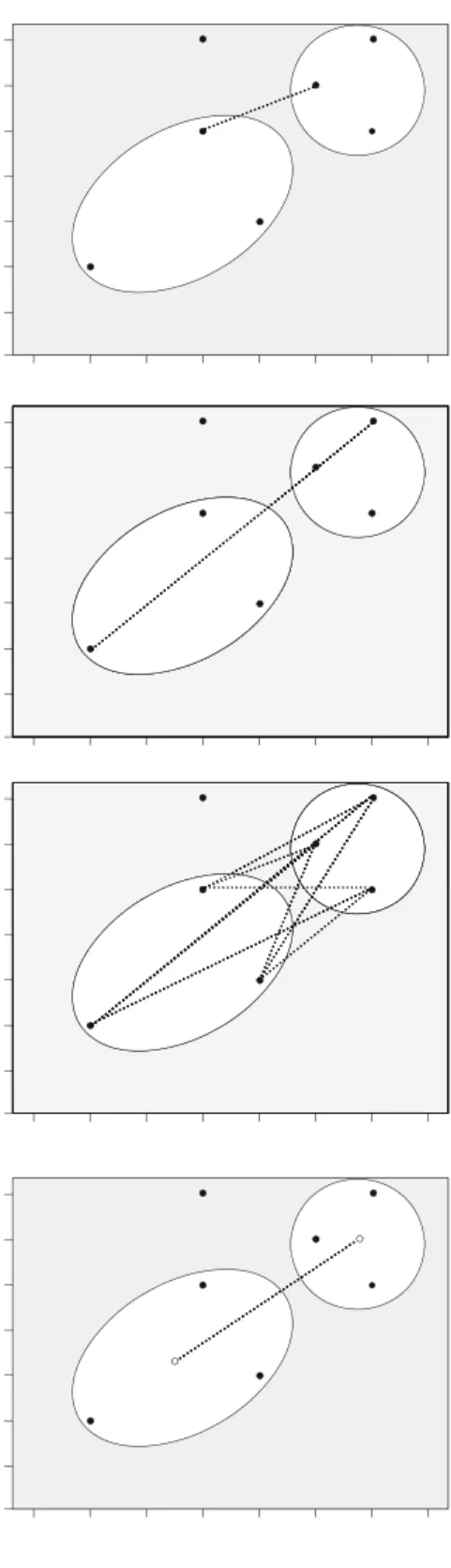
After having chosen the distance or similarity measure, we need to decide which clustering algorithm to apply. There are several agglomerative procedures and they can be distinguished by the way they define the distance from a newly formed cluster to a certain object, or to other clusters in the solution. The most popular agglomerative clustering procedures include the following:
l Single linkage (nearest neighbor): The distance between two clusters
corre-sponds to the shortest distance between any two members in the two clusters.
l Complete linkage (furthest neighbor): The oppositional approach to single
linkage assumes that the distance between two clusters is based on the longest distance between any two members in the two clusters.
l Average linkage: The distance between two clusters is defined as the average
distance between all pairs of the two clusters’ members.
l Centroid: In this approach, the geometric center (centroid) of each cluster is computed first. The distance between the two clusters equals the distance bet-ween the two centroids.
Figures 9.5–9.8 illustrate these linkage procedures for two randomly framed
Fig. 9.5 Single linkage
Fig. 9.6 Complete linkage
Fig. 9.7 Average linkage
Each of these linkage algorithms can yield totally different results when used on the same dataset, as each has its specific properties. As the single linkage algorithm is based on minimum distances, it tends to form one large cluster with the other clusters containing only one or few objects each. We can make use of this “chaining effect” to detect outliers, as these will be merged with the remain-ing objects – usually at very large distances – in the last steps of the analysis. Generally, single linkage is considered the most versatile algorithm. Conversely, the complete linkage method is strongly affected by outliers, as it is based on maximum distances. Clusters produced by this method are likely to be rather compact and tightly clustered. The average linkage and centroid algorithms tend to produce clusters with rather low within-cluster variance and similar sizes. However, both procedures are affected by outliers, though not as much as complete linkage.
Another commonly used approach in hierarchical clustering isWard’s method.
This approach does not combine the two most similar objects successively. Instead, those objects whose merger increases the overall within-cluster variance to the smallest possible degree, are combined. If you expect somewhat equally sized clusters and the dataset does not include outliers, you should always use Ward’s method.
To better understand how a clustering algorithm works, let’s manually examine some of the single linkage procedure’s calculation steps. We start off by looking at
the initial (Euclidean) distance matrix in Table9.3. In the very first step, the two
objects exhibiting the smallest distance in the matrix are merged. Note that we always merge those objects with the smallest distance, regardless of the clustering procedure (e.g., single or complete linkage). As we can see, this happens to two
pairs of objects, namely B and C (d(B, C)¼1.414), as well as C and E (d(C, E)¼
1.414). In the next step, we will see that it does not make any difference whether we first merge the one or the other, so let’s proceed by forming a new cluster, using objects B and C.
Having made this decision, we then form a new distance matrix by considering the single linkage decision rule as discussed above. According to this rule, the distance from, for example, object A to the newly formed cluster is the minimum of d(A, B) and d(A, C). As d(A, C) is smaller than d(A, B), the distance from A to the newly formed cluster is equal to d(A, C); that is, 2.236. We also compute the distances from cluster [B,C] (clusters are indicated by means of squared brackets) to all other objects (i.e. D, E, F, G) and simply copy the remaining distances – such as d(E, F) – that the previous clustering has not affected. This yields the distance
matrix shown in Table9.6.
Continuing the clustering procedure, we simply repeat the last step by merging the objects in the new distance matrix that exhibit the smallest distance (in this case, the newly formed cluster [B, C] and object E) and calculate the distance from this
cluster to all other objects. The result of this step is described in Table9.7.
Try to calculate the remaining steps yourself and compare your solution with the
By following the single linkage procedure, the last steps involve the merger of cluster [A,B,C,D,E,F] and object G at a distance of 3.162. Do you get the same results? As you can see, conducting a basic cluster analysis manually is not that hard at all – not if there are only a few objects in the dataset.
A common way to visualize the cluster analysis’s progress is by drawing a
dendrogram, which displays the distance level at which there was a combination
of objects and clusters (Fig.9.9).
We read the dendrogram from left to right to see at which distance objects have been combined. For example, according to our calculations above, objects B, C, and E are combined at a distance level of 1.414.
Table 9.6 Distance matrix after first clustering step (single linkage)
Objects A B, C D E F G A 0 B, C 2.236 0 D 2 2.236 0 E 3.606 1.414 3 0 F 4.123 3.162 2.236 2.828 0 G 5.385 5.657 3.606 5.831 3.162 0
Table 9.7 Distance matrix after second clustering step (single linkage)
Objects A B, C, E D F G A 0 B, C, E 2.236 0 D 2 2.236 0 F 4.123 2.828 2.236 0 G 5.385 5.657 3.606 3.162 0
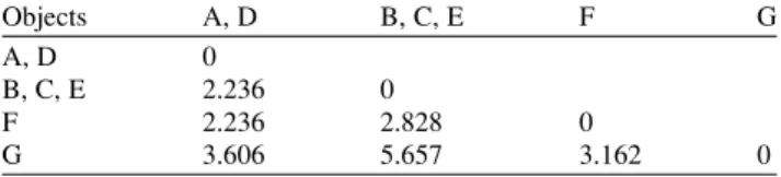
Table 9.8 Distance matrix after third clustering step (single linkage)
Objects A, D B, C, E F G
A, D 0
B, C, E 2.236 0
F 2.236 2.828 0
G 3.606 5.657 3.162 0
Table 9.9 Distance matrix after fourth clustering step (single linkage)
Objects A, B, C, D, E F G
A, B, C, D, E 0
F 2.236 0
G 3.606 3.162 0
Table 9.10 Distance matrix after fifth clustering step (single linkage)
Objects A, B, C, D, E, F G
A, B, C, D, E, F 0
Decide on the Number of Clusters
An important question we haven’t yet addressed is how to decide on the number of clusters to retain from the data. Unfortunately, hierarchical methods provide only very limited guidance for making this decision. The only meaningful indicator relates to the distances at which the objects are combined. Similar to factor analysis’s scree plot, we can seek a solution in which an additional combination of clusters or objects would occur at a greatly increased distance. This raises the issue of what a great distance is, of course.
One potential way to solve this problem is to plot the number of clusters on the x-axis (starting with the one-cluster solution at the very left) against the distance at which objects or clusters are combined on the y-axis. Using this plot, we then search
for the distinctive break (elbow). SPSS does not produce this plot automatically –
you have to use the distances provided by SPSS to draw a line chart by using a common spreadsheet program such as Microsoft Excel.
Alternatively, we can make use of the dendrogram which essentially carries the same information. SPSS provides a dendrogram; however, this differs slightly from
the one presented in Fig.9.9. Specifically, SPSS rescales the distances to a range
of 0–25; that is, the last merging step to a one-cluster solution takes place at a (rescaled) distance of 25. The rescaling often lengthens the merging steps, thus making breaks occurring at a greatly increased distance level more obvious.
Despite this, this distance-based decision rule does not work very well in all cases. It is often difficult to identify where the break actually occurs. This is also the case in our example above. By looking at the dendrogram, we could justify a two-cluster solution ([A,B,C,D,E,F] and [G]), as well as a five-cluster solution ([B,C,E], [A], [D], [F], [G]). B C E A D F G 3 2 1 0 Distance Fig. 9.9 Dendrogram
Research has suggested several other procedures for determining the number of
clusters in a dataset. Most notably, thevariance ratio criterion(VRC) by Calinski
and Harabasz (1974) has proven to work well in many situations.8For a solution
withnobjects andksegments, the criterion is given by:
VRCk¼ ðSSB=ðk1ÞÞ=ðSSW=ðnkÞÞ;
whereSSBis the sum of the squares between the segments andSSWis the sum of the
squares within the segments. The criterion should seem familiar, as this is nothing
but the F-value of a one-way ANOVA, with k representing the factor levels.
Consequently, the VRC can easily be computed using SPSS, even though it is not readily available in the clustering procedures’ outputs.
To finally determine the appropriate number of segments, we computeokfor
each segment solution as follows:
ok¼ðVRCkþ1VRCkÞ ðVRCkVRCk1Þ:
In the next step, we choose the number of segmentskthat minimizes the value in
ok. Owing to the term VRCk1, the minimum number of clusters that can be
selected is three, which is a clear disadvantage of the criterion, thus limiting its application in practice.
Overall, the data can often only provide rough guidance regarding the number of clusters you should select; consequently, you should rather revert to practical considerations. Occasionally, you might have a priori knowledge, or a theory on which you can base your choice. However, first and foremost, you should ensure that your results are interpretable and meaningful. Not only must the number of clusters be small enough to ensure manageability, but each segment should also be large enough to warrant strategic attention.
Partitioning Methods: k-means
Another important group of clustering procedures are partitioning methods. As with hierarchical clustering, there is a wide array of different algorithms; of these, the
k-means procedureis the most important one for market research.9The k-means algorithm follows an entirely different concept than the hierarchical methods discussed before. This algorithm is not based on distance measures such as Euclidean distance or city-block distance, but uses the within-cluster variation as a
8Milligan and Cooper (1985) compare various criteria.
9Note that the k-means algorithm is one of the simplest non-hierarchical clustering methods. Several extensions, such as k-medoids (Kaufman and Rousseeuw2005) have been proposed to handle problematic aspects of the procedure. More advanced methods include finite mixture models (McLachlan and Peel2000), neural networks (Bishop2006), and self-organizing maps (Kohonen1982). Andrews and Currim (2003) discuss the validity of some of these approaches.
measure to form homogenous clusters. Specifically, the procedure aims at segmenting the data in such a way that the within-cluster variation is minimized. Consequently, we do not need to decide on a distance measure in the first step of the analysis.
The clustering process starts by randomly assigning objects to a number of
clusters.10 The objects are then successively reassigned to other clusters to
mini-mize the within-cluster variation, which is basically the (squared) distance from each observation to the center of the associated cluster. If the reallocation of an object to another cluster decreases the within-cluster variation, this object is reas-signed to that cluster.
With the hierarchical methods, an object remains in a cluster once it is assigned to it, but with k-means, cluster affiliations can change in the course of the clustering process. Consequently, k-means does not build a hierarchy as described before
(Fig.9.3), which is why the approach is also frequently labeled as non-hierarchical.
For a better understanding of the approach, let’s take a look at how it works in
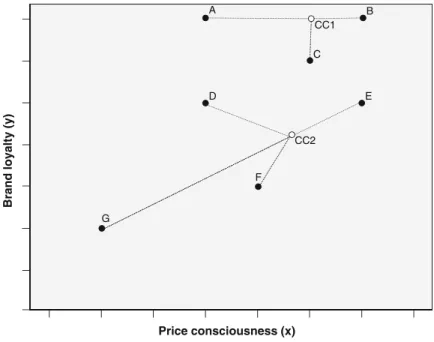
practice. Figs.9.10–9.13illustrate the k-means clustering process.
Prior to analysis, we have to decide on the number of clusters. Our client could, for example, tell us how many segments are needed, or we may know from previous research what to look for. Based on this information, the algorithm randomly selects a center for each cluster (step 1). In our example, two cluster centers are randomly
initiated, which CC1 (first cluster) and CC2 (second cluster) in Fig. 9.10
B A CC1 D E C CC2 F
Brand loyalty (y)
G
Price consciousness (x) Fig. 9.10 k-means procedure (step 1)
B A CC1 C D E CC2 F Brand loyalty (y ) G Price consciousness (x) Fig. 9.11 k-means procedure (step 2)
B A CC1 CC1′ C CC2 F CC2′ Brand loyalty (y ) G Price consciousness (x) E D
represent.11After this (step 2), Euclidean distances are computed from the cluster centers to every single object. Each object is then assigned to the cluster center with
the shortest distance to it. In our example (Fig. 9.11), objects A, B, and C are
assigned to the first cluster, whereas objects D, E, F, and G are assigned to the second. We now have our initial partitioning of the objects into two clusters.
Based on this initial partition, each cluster’s geometric center (i.e., its centroid) is computed (third step). This is done by computing the mean values of the objects contained in the cluster (e.g., A, B, C in the first cluster) regarding each of the variables
(price consciousness and brand loyalty). As we can see in Fig.9.12, both clusters’
centers now shift into new positions (CC1’ for the first and CC2’ for the second cluster). In the fourth step, the distances from each object to the newly located cluster centers are computed and objects are again assigned to a certain cluster on the basis of their minimum distance to other cluster centers (CC1’ and CC2’). Since the cluster centers’ position changed with respect to the initial situation in the first step, this could lead to a different cluster solution. This is also true of our example, as object E is now – unlike in the initial partition – closer to the first cluster center (CC1’) than to the second (CC2’). Consequently, this object is now assigned to the
first cluster (Fig. 9.13). The k-means procedure now repeats the third step and
re-computes the cluster centers of the newly formed clusters, and so on. In other B A CC1′ C D F CC2′ Brand loyalty (y ) G Price consciousness (x) E
Fig. 9.13 k-means procedure (step 4)
11Conversely, SPSS always sets one observation as the cluster center instead of picking some random point in the dataset.
words, steps 3 and 4 are repeated until a predetermined number of iterations are reached, or convergence is achieved (i.e., there is no change in the cluster affiliations). Generally, k-means is superior to hierarchical methods as it is less affected by outliers and the presence of irrelevant clustering variables. Furthermore, k-means can be applied to very large datasets, as the procedure is less computationally demanding than hierarchical methods. In fact, we suggest definitely using k-means for sample sizes above 500, especially if many clustering variables are used. From a strictly statistical viewpoint, k-means should only be used on interval or ratio-scaled data as the procedure relies on Euclidean distances. However, the procedure is routinely used on ordinal data as well, even though there might be some distortions.
One problem associated with the application of k-means relates to the fact that the researcher has to pre-specify the number of clusters to retain from the data. This makes k-means less attractive to some and still hinders its routine application in practice. However, the VRC discussed above can likewise be used for k-means
clustering (an application of this index can be found in the8Web Appendix!
Chap. 9). Another workaround that many market researchers routinely use is to
apply a hierarchical procedure to determine the number of clusters and k-means
afterwards.12This also enables the user to find starting values for the initial cluster
centers to handle a second problem, which relates to the procedure’s sensitivity to the initial classification (we will follow this approach in the example application).
Two-Step Clustering
We have already discussed the issue of analyzing mixed variables measured on
different scale levels in this chapter. The two-step cluster analysis developed
by Chiu et al. (2001) has been specifically designed to handle this problem. Like
k-means, the procedure can also effectively cope with very large datasets. The name two-step clustering is already an indication that the algorithm is based on a two-stage approach: In the first stage, the algorithm undertakes a procedure that is very similar to the k-means algorithm. Based on these results, the two-step procedure conducts a modified hierarchical agglomerative clustering procedure that combines the objects sequentially to form homogenous clusters. This is done by building a so-called cluster feature tree whose “leaves” represent distinct objects in the dataset. The procedure can handle categorical and continuous variables simul-taneously and offers the user the flexibility to specify the cluster numbers as well as the maximum number of clusters, or to allow the technique to automatically choose the number of clusters on the basis of statistical evaluation criteria. Likewise, the procedure guides the decision of how many clusters to retain from the data by
calculating measures-of-fit such asAkaike’s Information Criterion (AIC)orBayes
Information Criterion (BIC). Furthermore, the procedure indicates each variable’s importance for the construction of a specific cluster. These desirable features make the somewhat less popular two-step clustering a viable alternative to the traditional methods. You can find a more detailed discussion of the two-step clustering
procedure in the8Web Appendix (!Chap.9), but we will also apply this method
in the subsequent example.
Validate and Interpret the Cluster Solution
Before interpreting the cluster solution, we have to assess the solution’s stability and validity. Stability is evaluated by using different clustering procedures on the same data and testing whether these yield the same results. In hierarchical cluster-ing, you can likewise use different distance measures. However, please note that it is common for results to change even when your solution is adequate. How much variation you should allow before questioning the stability of your solution is a matter of taste. Another common approach is to split the dataset into two halves and to thereafter analyze the two subsets separately using the same parameter settings. You then compare the two solutions’ cluster centroids. If these do not differ significantly, you can presume that the overall solution has a high degree of stability. When using hierarchical clustering, it is also worthwhile changing the order of the objects in your dataset and re-running the analysis to check the results’ stability. The results should not, of course, depend on the order of the dataset. If they do, you should try to ascertain if any obvious outliers may influence the results of the change in order.
Assessing the solution’s reliability is closely related to the above, as reliability refers to the degree to which the solution is stable over time. If segments quickly change their composition, or its members their behavior, targeting strategies are likely not to succeed. Therefore, a certain degree of stability is necessary to ensure that marketing strategies can be implemented and produce adequate results. This can be evaluated by critically revisiting and replicating the clustering results at a later point in time.
To validate the clustering solution, we need to assess its criterion validity. In research, we could focus on criterion variables that have a theoretically based relationship with the clustering variables, but were not included in the analysis. In market research, criterion variables usually relate to managerial outcomes such as the sales per person, or satisfaction. If these criterion variables differ signifi-cantly, we can conclude that the clusters are distinct groups with criterion validity.
To judge validity, you should also assess face validity and, if possible, expert validity. While we primarily consider criterion validity when choosing clustering variables, as well as in this final step of the analysis procedure, the assessment of face validity is a process rather than a single event. The key to successful segmentation is to critically revisit the results of different cluster analysis set-ups (e.g., by using
different algorithms on the same data) in terms of managerial relevance. This under-lines the exploratory character of the method. The following criteria will help you
make an evaluation choice for a clustering solution (Dibb1999; Tonks2009; Kotler
and Keller 2009).
l Substantial: The segments are large and profitable enough to serve.
l Accessible: The segments can be effectively reached and served, which requires
them to be characterized by means of observable variables.
l Differentiable: The segments can be distinguished conceptually and respond differently to different marketing-mix elements and programs.
l Actionable: Effective programs can be formulated to attract and serve the segments.
l Stable: Only segments that are stable over time can provide the necessary grounds for a successful marketing strategy.
l Parsimonious: To be managerially meaningful, only a small set of substantial
clusters should be identified.
l Familiar: To ensure management acceptance, the segments composition should
be comprehensible.
l Relevant: Segments should be relevant in respect of the company’s competencies
and objectives.
l Compactness: Segments exhibit a high degree of within-segment homogeneity
and between-segment heterogeneity.
l Compatibility: Segmentation results meet other managerial functions’
require-ments.
The final step of any cluster analysis is the interpretation of the clusters. Interpreting clusters always involves examining the cluster centroids, which are the clustering variables’ average values of all objects in a certain cluster. This step is of the utmost importance, as the analysis sheds light on whether the segments are conceptually distinguishable. Only if certain clusters exhibit significantly different means in these variables are they distinguishable – from a data perspective, at least. This can easily be ascertained by comparing the clusters with independent t-tests
samples or ANOVA (see Chap.6).
By using this information, we can also try to come up with a meaningful name or label for each cluster; that is, one which adequately reflects the objects in the cluster. This is usually a very challenging task. Furthermore, clustering variables are frequently unobservable, which poses another problem. How can we decide to which segment a new object should be assigned if its unobservable characteristics, such as personality traits, personal values or lifestyles, are unknown? We could obviously try to survey these attributes and make a decision based on the clustering variables. However, this will not be feasible in most situations and researchers therefore try to identify observable variables that best mirror the partition of the objects. If it is possible to identify, for example, demographic variables leading to a very similar partition as that obtained through the segmentation, then it is easy to assign a new object to a certain segment on the basis of these demographic
characteristics. These variables can then also be used to characterize specific
segments, an action commonly calledprofiling.
For example, imagine that we used a set of items to assess the respondents’ values and learned that a certain segment comprises respondents who appreciate self-fulfillment, enjoyment of life, and a sense of accomplishment, whereas this is not the case in another segment. If we were able to identify explanatory variables such as gender or age, which adequately distinguish these segments, then we could partition a new person based on the modalities of these observable variables whose traits may still be unknown.
Table9.11summarizes the steps involved in a hierarchical and k-means clustering.
We also introduce steps related to two-step clustering which we will further introduce in the subsequent example.
While companies often develop their own market segments, they frequently use standardized segments, which are based on established buying trends, habits, and customers’ needs and have been specifically designed for use by many products in mature markets. One of the most popular approaches is the PRIZM lifestyle segmentation system developed by Claritas Inc., a leading market research com-pany. PRIZM defines every US household in terms of 66 demographically and behaviorally distinct segments to help marketers discern those consumers’ likes, dislikes, lifestyles, and purchase behaviors.
Visit the Claritas website and flip through the various segment profiles. By entering a 5-digit US ZIP code, you can also find a specific neighborhood’s top five lifestyle groups.
One example of a segment is “Gray Power,” containing middle-class, home-owning suburbanites who are aging in place rather than moving to retirement communities. Gray Power reflects this trend, a segment of older, midscale singles and couples who live in quiet comfort.
Table 9.11 Steps involved in carrying out a factor analysis in SPSS
Theory Action
Research problem
Identification of homogenous groups of objects in a population
Select clustering variables that should be used to form segments
Select relevant variables that potentially exhibit high degrees of criterion validity with regard to a specific managerial objective.
Requirements
Sufficient sample size Make sure that the relationship between objects and clustering variables is reasonable (rough guideline: number of observations should be at least 2m, wheremis the number of clustering variables). Ensure that the sample size is large enough to guarantee substantial segments. Low levels of collinearity among the variables
▸
Analyze▸
Correlate▸
BivariateEliminate or replace highly correlated variables (correlation coefficients>0.90).
Specification
Choose the clustering procedure If there is a limited number of objects in your dataset or you do not know the number of clusters:
▸
Analyze▸
Classify▸
Hierarchical Cluster If there are many observations (>500) in yourdataset and you have a priori knowledge regarding the number of clusters:
▸
Analyze▸
Classify▸
K-Means Cluster If there are many observations in your dataset andthe clustering variables are measured on different scale levels:
▸
Analyze▸
Classify▸
Two-Step Cluster Select a measure of similarity or dissimilarity(only hierarchical and two-step clustering)
Hierarchical methods:
▸
Analyze▸
Classify▸
Hierarchical Cluster▸
Method▸
MeasureDepending on the scale level, select the measure; convert variables with multiple categories into a set of binary variables and use matching coefficients; standardize variables if necessary (on a range of 0 to 1 or1 to 1).
Two-step clustering:
▸
Analyze▸
Classify▸
Two-Step Cluster▸
Distance MeasureUse Euclidean distances when all variables are continuous; for mixed variables, use log-likelihood.
Choose clustering algorithm
(only hierarchical clustering)
▸
Analyze
▸
Classify▸
Hierarchical Cluster▸
Method▸
Cluster MethodUse Ward’s method if equally sized clusters are expected and no outliers are present. Preferably use single linkage, also to detect outliers.
Decide on the number of clusters Hierarchical clustering: Examine the dendrogram:
▸
Analyze▸
Classify▸
Hierarchical Cluster▸
Plots▸
DendrogramTable 9.11 (continued)
Theory Action
Draw a scree plot (e.g., using Microsoft Excel) based on the coefficients in the agglomeration schedule.
Compute the VRC using the ANOVA procedure:
▸
Analyze▸
Compare Means▸
One-WayANOVA
Move the cluster membership variable in the Factorbox and the clustering variables in the Dependent Listbox.
Compute VRC for each segment solution and compare values.
k-means:
Run a hierarchical cluster analysis and decide on the number of segments based on a dendrogram or scree plot; use this information to run k-means with k clusters.
Compute the VRC using the ANOVA procedure:
▸
Analyze▸
Classify▸
K-Means Cluster▸
Options
▸
ANOVA table; Compute VRC for each segment solution and compare values. Two-step clustering:Specify the maximum number of clusters:
▸
Analyze▸
Classify▸
Two-Step Cluster▸
Number of ClustersRun separate analyses using AIC and, alternatively, BIC as clustering criterion:
▸
Analyze▸
Classify▸
Two-Step Cluster▸
Clustering Criterion
Examine the auto-clustering output. Validate and interpret the cluster solution
Assess the solution’s stability Re-run the analysis using different clustering procedures, algorithms or distance measures. Split the datasets into two halves and compute the
clustering variables’ centroids; compare centroids for significant differences (e.g., independent-samples t-test or one-way ANOVA).
Change the ordering of objects in the dataset (hierarchical clustering only).
Assess the solution’s reliability Replicate the analysis using a separate, newly collected dataset.
Assess the solution’s validity Criterion validity:
Evaluate whether there are significant differences between the segments with regard to one or more criterion variables.
Face and expert validity:
Segments should be substantial, accessible, differentiable, actionable, stable,
parsimonious, familiar and relevant. Segments should exhibit high degrees of within-segment homogeneity and between-segment
heterogeneity. The segmentation results should meet the requirements of other managerial functions.
Example
Silicon-Valley-based Tesla Motors Inc. (http://www.teslamotors.com) is an
auto-mobile startup company focusing on the production of high performance electrical vehicles with exceptional design, technology, performance, and efficiency. Having reported the 500th delivery of its roadster in June 2009, the company decided to focus more strongly on the European market. However, as the company has only limited experience in the European market, which has different characteristics than that of the US, it asked a market research firm to provide a segmentation concept. Consequently, the market research firm gathered data from major car manufacturers on the following car characteristics, all of which have been measured on a ratio scale (variable names in parentheses):
l Engine displacement (displacement)
l Turning moment in Nm (moment)
l Horsepower (horsepower)
l Length in mm (length)
l Width in mm (width)
l Net weight in kg (weight)
l Trunk volume in liters (trunk)
l Maximum speed in km/h (speed)
l Acceleration 0–100 km/h in seconds (acceleration)
Table 9.11 (continued)
Theory Action
Interpret the cluster solution Examine cluster centroids and assess whether these differ significantly from each other (e.g., by means of t-tests or ANOVA; see Chap.6). Identify names or labels for each cluster and
characterize each cluster by means of observable variables, if necessary (cluster profiling).
The pretest sample of 15, randomly taken, cars is shown in Fig.9.14. In practice, clustering is done on much larger samples but we use a small sample size to illustrate the clustering process. Keep in mind that in this example, the ratio between the objects and clustering variables is much too small. The dataset used iscars.sav(8Web Appendix!Chap.9).
In the next step, we will run several different clustering procedures on the basis of these nine variables. We first apply a hierarchical cluster analysis based on Euclidean distances, using the single linkage method. This will help us determine a suitable number of segments, which we will use as input for a subsequent k-means clustering. Finally, we will run a two-step cluster analysis using SPSS.
Before we start with the clustering process, we have to examine the variables for substantial collinearity. Just by looking at the variable set, we suspect that there are some highly correlated variables in our dataset. For example, we expect rather high
correlations betweenspeedandacceleration. To determine this, we run a bivariate
correlation analysis by clicking
▸
Analyze▸
Correlate▸
Bivariate, which will opena dialog box similar to that in Fig.9.15. Enter all variables into theVariablesbox
and select the box Pearson(under Correlation Coefficients) because these are
continuous variables.
The correlation matrix in Table 9.12 supports our expectations – there are
several variables that have high correlations.Displacementexhibits high (absolute)
correlation coefficients withhorsepower,speed, andacceleration, with values well
above 0.90, indicating possible collinearity issues. Similarly,horsepoweris highly
correlated withspeedandacceleration. Likewise,lengthshows a high degree of
correlation withwidth,weight, andtrunk.
A potential solution to this problem would be to run a factor analysis and perform a cluster analysis on the resulting factor scores. Since the factors obtained are, by definition, independent, this would allow for an effective handling of the collinearity issue. However, as this approach is associated with several problems (see discussion above) and as there are only several variables in our data set,
we should reduce the variables, for example, by omittingdisplacement,horsepower,
andlengthfrom the subsequent analyses. The remaining variables still provide a sound basis for carrying out cluster analysis.
To run the hierarchical clustering procedure, click on
▸
Analyze▸
Classify▸
Hierarchical Cluster, which opens a dialog box similar to Fig.9.16.
Move the variablesmoment,width,weight,trunk,speed, andaccelerationinto
theVariable(s)box and specifynameas the labeling variable (boxLabel Cases
by). TheStatistics option gives us the opportunity to request the distance matrix
(labeled proximity matrix in this case) and the agglomeration schedule, which provides information on the objects being combined at each stage of the clustering process. Furthermore, we can specify the number or range of clusters to retain from the data. As we do not yet know how many clusters to retain, just check the box
Agglomeration scheduleand continue.
UnderPlots, we choose to display a dendrogram, which graphically displays the
distances at which objects and clusters are joined. Also ensure you select the icicle diagram (for all clusters), which is yet another graph for displaying clustering solutions.
The optionMethodallows us to specify the cluster method (e.g., single linkage
or Ward’s method), the distance measure (e.g., Chebychev distance or the Jaccard coefficient), and the type of standardization of values. In this example, we use the
single linkage method (Nearest neighbor) based onEuclidean distances. Since
the variables are measured on different levels (e.g., speed versus weight), make sure
to standardize the variables, using, for example, theRange1 to 1(by variable) in
theTransform Valuesdrop-down list.
Table 9.12 Correlation matrix Correlations displacement moment horsepower length width weight trunk speed acceleration displacement Pearson Correlation 1 .875 ** .983 ** .657 ** .764 ** .768 ** .470 .967 ** –.969 ** Sig. (2-tailed) .000 .000 .008 .001 .001 .077 .000 .000 N1 5 1 5 1 5 1 5 1 5 1 5 1 5 1 5 1 5 moment Pearson Correlation .875 ** 1 .847 ** .767 ** .766 ** .862 ** .691 ** .859 ** –.861 ** Sig. (2-tailed) .000 .000 .001 .001 .000 .004 .000 .000 N 1 5 1 5 1 5 1 5 1 51 5 1 51 5 1 5 horsepower Pearson Correlation .983 ** .847 ** 1 .608 * .732 ** .714 ** .408 .968 ** –.961 ** Sig. (2-tailed) .000 .000 .016 .002 .003 .131 .000 .000 N1 5 1 5 1 5 1 5 1 5 1 5 1 5 1 5 1 5 length Pearson Correlation .657 ** .767 ** .608 * 1 .912 ** .921 ** .934 ** .741 ** –.714 ** Sig. (2-tailed) .008 .001 .016 .000 .000 .000 .002 .003 N1 5 1 5 1 5 1 5 1 5 1 5 1 5 1 5 1 5 width Pearson Correlation .764 ** .766 ** .732 ** .912 ** 1 .884 ** .783 ** .819 ** –.818 ** Sig. (2-tailed) .001 .001 .002 .000 .000 .001 .000 .000 N1 5 1 5 1 5 1 5 1 5 1 5 1 5 1 5 1 5 weight Pearson Correlation .768 ** .862 ** .714 ** .921 ** .884 ** 1 .785 ** .778 ** –.763 ** Sig. (2-tailed) .001 .000 .003 .000 .000 .001 .001 .001 N1 5 1 5 1 5 1 5 1 5 1 5 1 5 1 5 1 5 trunk Pearson Correlation .470 .691 ** .408 .934 ** .783 ** .785 ** 1 .579 * –.552 * Sig. (2-tailed) .077 .004 .131 .000 .001 .001 .024 .033 N1 5 1 5 1 5 1 5 1 5 1 5 1 5 1 5 1 5 speed Pearson Correlation .967 ** .859 ** .968 ** .741 ** .819 ** .778 ** .579 * 1 –.971 ** Sig. (2-tailed) .000 .000 .000 .002 .000 .001 .024 .000 N1 5 1 5 1 5 1 5 1 5 1 5 1 5 1 5 1 5 acceleration Pearson Correlation –.969 ** –.861 ** –.961 ** –.714 ** –.818 ** –.763 ** –.552 * –.971 ** 1 Sig. (2-tailed) .000 .000 .000 .003 .000 .001 .033 .000 N 1 5 1 5 1 5 1 5 1 51 5 1 51 5 1 5
**. Correlation is significant at the 0.01 level (2-tailed). *. Correlation is si
g
Lastly, the Save option enables us to save cluster memberships for a single solution or a range of solutions. Saved variables can then be used in subsequent analyses to explore differences between groups. As a start, we will skip this option,
so continue and click onOKin the main menu.
Fig. 9.16 Hierarchical cluster analysis dialog box
Table 9.13 Agglomeration schedule
Agglomeration Schedule
Stage Cluster Combined
Coefficients
Stage Cluster First Appears
Next Stage
Cluster 1 Cluster 2 Cluster 1 Cluster 2
1 5 6 .149 0 0 2 2 5 7 .184 1 0 3 3 4 5 .201 0 2 5 4 14 15 .213 0 0 6 5 3 4 .220 0 3 8 6 13 14 .267 0 4 11 7 11 12 .321 0 0 9 8 2 3 .353 0 5 10 9 10 11 .357 0 7 11 10 1 2 .389 0 8 14 11 10 13 .484 9 6 13 12 8 9 .575 0 0 13 13 8 10 .618 12 11 14 14 1 8 .910 10 13 0
First, we take a closer look at the agglomeration schedule (Table9.13), which displays the objects or clusters combined at each stage (second and third column) and the distances at which this merger takes place. For example, in the first stage, objects 5 and 6 are merged at a distance of 0.149. From here onward, the resulting cluster is labeled as indicated by the first object involved in this merger, which is object 5. The last column on the very right tells you in which stage of the algorithm this cluster will appear next. In this case, this happens in the second step, where it is merged with object 7 at a distance of 0.184. The resulting cluster is still labeled 5, and so on. Similar information is provided by the icicle diagram shown in
Fig.9.17. Its name stems from the analogy to rows of icicles hanging from the eaves
of a house. The diagram is read from the bottom to the top, therefore the columns correspond to the objects being clustered, and the rows represent the number of clusters.
As described earlier, we can us