Light Fields Reconstructing Geometry and Reflectance Properties

(1)

Dissertation

submitted to the

Combined Faculties for the

Natural Sciences and for Mathematics

of the Ruperto-Carola University of Heidelberg, Germany

for the degree of

Doctor of Natural Sciences

put forward by

M.Sc. Marcel Gutsche

born in Frankfurt am Main, Germany

Date of oral exam: July, 16th 2018

(2)

(3)

Light Fields

Reconstructing Geometry and

Reflectance Properties

(4)

PD Dr. rer. nat. Christoph Garbe

Prof. Dr. rer. nat. Karl-Heinz Brenner

(5)

Zusammenfassung: Maschinelles Sehen spielt eine wichtige Rolle im Fortschritt der Automatisierung und der Digitalisierung in unserer Gesellschaft. Die Konstruktion exakter 3D-Modelle ist dabei eine zentrale Herausforderung. Das Lichtfeld beschreibt dabei für jeden Raumpunkt und jeden Raumwinkel die Lichtstrahlen. Diese Datenfülle die Lichtfelder bieten erlaubt präzise Tiefenschätzungen, erfordert aber auch die Entwicklung neuer Algorithmen.

Insbesondere spekulare Reflexionen bereiten existierenden Algorithmen Probleme. Der Grund dafür liegt in der vereinfachenden Annahme der meisten Algorithmen, dass die Helligkeit eines Objektpunktes konstant über verschiedene Ansichten bleibt. Die meisten Oberflächen erzeugen teilweise spekulare Reflektionen, was bei der Erstellung von Tiefenkarten berücksichti-gen werden muss.

In dieser Arbeit entwickeln wir verbesserte Algorithmen, die basierend auf Glanzlichtern die Oberflächenneigung schätzen. Dazu werden Epipolarbilder untersucht, die mit Lichtfeldaufbauten gewonnen werden. Lichtfelder bieten die Möglichkeit, Reflektionseigenschaften anhand von Intensitätsvariationen im Epipolarraum zu charakterisieren. Dieser Raum wird analysiert und mit der erwarteten Reflektanz verglichen, die mit Hilfe der Rendergleichung und verschiedenen bidirektionalen Reflektanzverteilungsfunktionen model-liert wird. Damit können nicht nur hoch präzise Oberflächennormalen und Tiefenkarten bestimmt werden, sondern auch Materialeigenschaften, welche in den Reflexionscharakteristiken enthalten sind.

Die Ergebnisse dieser Arbeit zeigen, dass mit den neuen Algorithmen genauere Tiefenkarten erstellt und zusätzlich Materialeigenschaften gemessen werden können, wenn mehrere Kameras in einem Lichtfeldaufbau benutzt werden.

(6)

Computer vision plays an important role in the progress of automation and digitalization of our society. One of the key challenges is the creation of accurate 3D representations of our environment. The rich information in light fields can enable highly accurate depth estimates, but requires the development of new algorithms.

Especially specular reflections pose a challenge for many reconstruction algorithms. This is due to the violation of the brightness consistency as-sumption, which only holds for Lambertian surfaces. Most surfaces are to some extent specular and an appropriate handling is central to avoid erro-neous depth maps.

In this thesis we explore the potential of using specular highlights to deter-mine the orientation of surfaces. To this end, we exadeter-mine epipolar images in light field set ups. In light field data, reflectance properties can be character-ized by intensity variations in the epipolar plane space. This space is analysed and compared to the expected reflectance, which is modelled using the render equation with different bidirectional reflection distribution functions.

This approach allows us to infer highly accurate surface normals and depth estimates. Furthermore, it reveals material properties encoded in the re-flectance by inspecting the intensity profile. Our results demonstrate the potential to increase the accuracy of the depth maps. Multiple cameras in a light field set up let us retrieve additional material properties encoded in the reflectance.

(7)

(8)

(9)

Acknowledgements

The research I did from 2014 to 2017 at the HCI in Heidelberg would not have been possible without all the great people I had the honour to work with.

Special thanks to Dr. Christoph Garbe, who made this dissertation possible and whose guidance and practical views were always valuable and encouraging. My gratitude also to Prof. Brenner, who agreed to be my second referee.

It was a pleasure working with the whole Light Field group / HD Vision Systems consisting of Christoph Garbe, Maximilian Diebold, Hendrik Schilling, Hamza Aziz, Alessandro Vianello, Sven Wanner and Wolfgang Mischler and our Ground Truth co-group Karsten Krispin, Katrin Honauer, Oliver Zendel, Alexan-der Brock and Burkhard Güssefeld. They did not only provide intelligent counsel in every subject related matter, but also were fantastic table football companions. I am thankful for the financial support to Prof. Katja Mombaur, Prof. Bernd Jähne and the HGS MathComp which allowed me to fully concentrate on the research.

I also thank my friends and my family for their unconditional support during all these years. Especially I want to thank Johann Brehmer, Merle Reinhart, Florian Dinger, Svenja Reith, Karsten Krispin and Hendrik Schilling for taking their time to proofread parts of this thesis.

(10)

(11)

1

Introduction

1.1 Motivation

One of the central challenges in computer vision is to recover the constituents of a 3D scene, including the geometry, the illumination and material properties. Disentangling all these elements from 2D images is commonly referred to as inverse rendering and a holy grail in computer vision.

These physical qualities of our surrounding surfaces, namely distance, orien-tation and material properties can be summarized by the term early vision, as stated by Poggio, Torre, and Koch [45]. In contrast, high-level vision tasks are more concerned with image semantics, meaning object detection, segmentation and classification. This thesis deals with the former, the reconstruction of dis-tance, orientation and material properties using light fields. Knowing all the constituents of a scene in terms of geometry, illumination and reflection proper-ties would tremendously help with a variety of tasks.

The applications of robust and precise reconstruction algorithms are almost endless and cover general navigation tasks through 3D space as well as content creation of real objects for more and more widespread 3D printers. There is currently a booming market for autonomous vehicles, such as drones, robots or self-driving cars, all in need for 3D maps of their surroundings to navigate safely.

(16)

In blockbuster films, computer generated imagery (CGI), based on 3D models of faces is used to generate digital make up with astonishing results, see Figure 1.1. Many high-level computer vision tasks that are challenging based on only 2D im-agery become almost trivial when additional depth information is incorporated, such as the segmentation of foreground and background objects. These findings have led to an enormous interest in research and camera development, such that even consumer devices are equipped with RBGD cameras, where additionally to the red, blue and green channel also depth is recorded. Recovering the underly-ing 3D world from 2D images is not only useful in a variety of applications, but it also provides interesting and challenging questions in the area of inverse render-ing, the process of recovering the geometry, material properties and illumination leading to the observed images. A hard problem, which is still unsolved.

In particular the effect of reflective materials on the appearance of objects is complex, handling these specular reflections is challenging. One key ingredient for the recovery of the 3D information is the relation of the same 3D point in, at least, two different views. The simplest approach is to assume constant brightness between the images. But many materials like metals or plastics do not reflect light equally in all directions. This aspect of non-uniform light distribution is discussed in great detail and possible solutions are addressed in this thesis.

The problem affects many applications. Examples include automated defect detection, where metallic surfaces are challenging to handle, and dental recon-struction techniques for the creation of custom-fit dentures. Non-uniform light distributions are the central topic of this thesis. We discuss it in detail and explore possible solutions.

An elegant way of representing and thinking about these non-uniform distri-butions is the light field representation. It describes the amount of light for each point in space and for each direction. In addition to the 3D geometry, this for-malism also describes the reflectance properties of the surfaces. There are many ways to capture part of the light field. For still scenes, gantries with a single

(17)

1.1 Motivation

(a) Digital make up based on the 3D location of a face featuring Davy Jones for Disney’s Pirates of the Caribbean. Image taken from [14].

(b) Parrot drone for creating 3D mod-els from above. Image taken from [43].

(c) 3D printer for metal objects. Image taken from [54].

(18)

mounted camera are used. Camera arrays allow for dynamic scenes, but require more sophisticated calibration procedures. Also, light field cameras for the con-sumer market are available. They provide the angular separation using mircolens arrays in front of the image sensor.

The huge amount of data in light fields is both a blessing and a challenge: while it is the reason behind their usefulness for many applications, it also makes them notoriously difficult to process. But according to Moore’s law, these computa-tional challenges will rather sooner than later pose a less urgent problem. Since many real world objects have specular characteristics, handling these phenom-ena correctly in the 3D reconstruction process helps to build robust navigation algorithms which do not falter in uncontrolled environments.

Motivated by the possible applications and the holy grail of perfect inverse rendering in mind, this thesis addresses the question of how to take advantage of specular highlights in the 3D reconstruction process, especially in combination with light field capture.

1.2 Related Work

A plethora of methods for 3D reconstruction have been established. Many meth-ods rely on triangulation, similar to the human vision system. Active systems are another important group of techniques. They are based on the duration be-tween emitting and receiving a signal. Examples include time of flight cameras (ToF [15]), radar, lidar, sonar and ultrasound. In contrast, passive systems do not emit a signal and only capture incoming light with one, two or more cameras. Methods have been proposed to estimate scene geometry from a single im-age [32, 33]. These techniques require either strong prior knowledge or use deep neural networks with a need for large training data sets. Due to their reliance

(19)

1.2 Related Work

on a single image they suffer from low accuracy and can only provide depth estimates up to a scale factor, also referred to as scale ambiguity.

Other interesting techniques use more images from a single view. In methods based on photometric stereo, images are acquired from the same position under changing light conditions. This approach, first proposed by Woodham [64], uses the information that the intensity varies with the angle between the surface normal and the direction of the incoming light. Using enough measurements with different light positions, the surface normal can be constrained to a unique solution. Other work also includes specular highlights in their photometric stereo approaches [22, 35].

Depth from defocus uses multiple views from the same position but with dif-ferent foci to estimate depth. The amount of blurring caused by the distance to the focal plane corresponds to the depth. This is especially used to get depth information in microscopy.

The methods presented in this thesis are based on 3D reconstruction from structured light fields. In general, light fields can be described by the plenoptic function [2], which describes the light as intensity as a function of both position and direction. It represents a high-dimensional function which contains all in-formation about the light emitted or reflected at an object surface. To reduce its dimensionality, Gortler et al. [18] and Levoy et al. [31] introduce the use of a 4D subset from the full light field which enables sampling of the light field using multiple cameras. Over the last years, state of the art light field scene reconstruction methods provide an increasing precision of depth estimates, even for difficult materials, at the cost of high runtimes [39, 65, 56, 13].

The accurate description of material properties is a topic often discussed in the computer graphics community with its interest in realistic rendering. Many models in particular for forward reflections have been developed. But typically they prioritize the aesthetics of the rendering as well as the computational

(20)

effi-ciency over the physical accuracy. In Chapter 2 we will discuss the theory behind material properties encoded in the bidirectional distribution function (BRDF) in more detail.

In the computer vision community specularities are often treated as undesired component. Hence, first publications were concerned with the detection of specu-lar highlights and the exclusion of such areas to avoid failure of algorithms based on Lambertian assumptions [4, 16, 29].

Early examinations of the information in specular highlights available for a moving observer with a static light source were conducted by Zissermanet al.[66]. They concluded that the information contained in the specular highlight by two or more images is sufficient to solve the convex/concave ambiguity, i.e. distin-guishing if a surface is bending inward or outward. However, they could not further constrain the curve generated by the moving observer on the surface. Ramamoorthi and Hanrahan [46] describe the reflected light fields as the con-volution of the light distribution with the BRDF, and the reconstruction of the scene geometry as deconvolution. Jin et al. [25] proposed another approach which utilizes a rank based cost function in a multi-view stereo setting. Other multi-view methods exploit multiple orientations in epipolar images, or similar features [10, 62, 11, 59].

Similar to the methods presented in this thesis is the work of Adatoet al. [1] but it is restricted to mirror like surfaces. They use the apparent displacement of the surface highlight in an optical flow frame work. Nairet al.[38] incorporate reflections and material properties in their stereo framework, but they do not actually handle lighting. Instead, they attribute all shading effects to the diffuse colour.

Oxholmet al.use a multi-view setup to infer geometry and reflectance proper-ties by means of a probabilistic model [42]. In contrast to the method presented here they need a full illumination model, whereas our method only needs the

(21)

1.3 Contribution

position of the strongest light source, which can be inferred by many different methods.

Jachnik et al. use methods based on self-localization and mapping algorithms (SLAM) to recover the specular and diffuse components of surfaces to apply augmented reality [23]. However, they assume planar surfaces and do not provide surface normal accuracies.

Wang et al. proposed a BRDF invariant theory to recover shape from light fields [60]. Their method generates depth and surface normals from input images, but relies on quadratic shape priors and smoothness constraints in neighbouring regions, whereas the method developed in this thesis provides pixel-wise depth and surface normal estimates.

1.3 Contribution

In this thesis, we develop methods for 3D reconstruction in the situation where the position of the light source and cameras are known. While we do not present a one-step solution for the holy grail of inverse rendering, which would include inferring the position of cameras and light sources, we make the following novel contributions:

• A novel algorithm for estimating surface normals based on the position of specular highlights in a light field camera set up.

• A procedure to estimate surface normals and BRDF parameters based on intensity variations in epipolar plane images.

• The integration of the surface normal and BRDF parameter estimator in general framework for deriving depth, material properties and surface

(22)

nor-mals.

1.4 Outline

In Chapter 2 the theoretical background for this thesis is provided. Starting from the mechanics of light transport, we explain the interaction processes, in particular the reflection on surfaces, and discuss the theory of 3D reconstruction based on light field data.

Chapter 3 is devoted to the light field acquisition process. We present the hardware used for gathering real data in this thesis, and show results for an optimal capturing setup.

In Chapter 4, we develop methods to reconstruct the surface normal from specular highlights in a cross shaped light field array. Here we only take the maximum position of the highlight for estimation. This leads to an interesting geometrical optimization problem.

In Chapter 5 we extend these techniques of by also taking into account the total intensity distribution. We demonstrate that this allows us to extract surface material properties in addition to the surface normal orientation.

Chapter 6 is the culmination of our work: We finally develop techniques to si-multaneously estimate the depth, the material properties and the surface normal orientation.

Chapter 7 gives a brief summary of this thesis and addresses possible future work.

(23)

2

Theory of Light Fields and

Reflectance

In this chapter an introduction about the theory of light transport and 3D re-constructions is presented. It does not go into all the details, but gives the basic insights and formulas which this thesis is build upon. A more throughout intro-duction and more details can be found in the books Digitale Bildverarbeitung, 6th revised and extended edition from Jähne [24] or in Multiple View Geometry in Computer Vision from Hartley and Zisserman[21]. Most of the explanations with regards to the bidirectional distribution functions (BRDFs) can be found in more detail in “An Overview of BRDF Models” from Montes Soldado and Ureña Almagro[37].

2.1 Light Transport

For the understanding of the image formation process the concepts of the inter-action between light and matter are highlighted. Depending on the material light will be partly transmitted, absorbed or reflected, see Figure 2.1. The reflection and transmission processes are governed by the Fresnel equations. They depend on the polarization of the light, the angle between the incoming light rayω_i_and

(24)

Re

ﬂ

ection

Surface

Absorption

Transmission

Figure 2.1: Light at an interface can be transmitted, absorbed or reflected. The total energy of the light is conserved. Second order effects, such as subsurface scattering, are not shown here.

(25)

2.1 Light Transport

refractive index n of the media at the interface. Additionally photons can be absorbed either by exciting vibrational modes of molecules or by exciting energy levels in the atom. We will ignore quantum specifics of light such as diffraction, but concentrate on the effects essential in geometrical optics. Before going into the details some radiometric terms are presented.

The energy of a photon is given by Qγ =

hc

λ, (2.1)

where h is Planck’s constant and c the speed of light. The flux or power is hence

Φ = dQ

dt . (2.2)

The irradiance is the flux per surface area, given as

E = dΦ

dA. (2.3)

For example the radiation of the Sun causes an irradiance above the Earth of 1.361 kW m−2_{, known as the solar constant.}

The radiance, given as

Le,Ω =

d2_Φ e

(26)

describes the amount of energy per time per unit area per solid angle and therefore has the units W sr−1_m−2_{. The factor} _A_cos_θ _{represents the projected} area under which the radiance is emitted, e.g.

Aprojected=A·(n·ω) = Acosθ, (2.5)

where n _{is the normalized surface normal of} _A _and ω _{the normalized direction}

of the in or outgoing light ray. The radiance is constant along geometrical lines of sight and does not fall off in contrast to the irradiance. This means that when a surface emits a radiance Le the same radiance will be received by an optical

system. However, this is not valid for point light sources, which are not fully resolvable in the imaging system. Here we would have to take the inverse square law into account.

We distinguish between diffuse and specular reflection. For a purely specular reflection the angle of the incident light is equal to the angle of reflection, e.g. a mirror. Diffuse reflection occurs on rough surfaces or due to scattering centers beneath the surface. If the light is distributed in all directions with equal likeli-hood we have a purely diffuse material. Almost all material have some mixture of a specular and a diffuse component. Plaster or marble are examples for very diffuse materials, while thin aluminium layers are strongly specular in the visible light. Diffuse surfaces are also called Lambertian reflectors, since they obey the Lambertian cosine law

Lo =

kd

π Licosθi, (2.6)

s where Li is the incident radiance and θi he angle between the surface normal and the incoming light, kd ∈ [0,1] is the diffuse albedo of the material and Lo the outgoing radiance. The factor of 1

π is due to the integration of the cosine

(27)

2.1 Light Transport

2.1.1 The Bidirectional Reflectance Distribution Function

Non Lambertian surfaces have a more complicated behaviour. Depending on the material we have larger reflection contributions towards certain directions, mostly in the direction of total reflection. This phenomenon is called specularity and in its most extreme form represents a perfect mirror, and all incoming rays obey the law of reflection. The bidirectional reflectance distribution function (BRDF) describes the ratio of reflected radiance Lr to the incoming irradiance

Ei, depending on the in and outgoing directions (ωi,ωo) of the light. It is defined as

fr(ωi,ωo) =

dLo(ωo)

Li(ωi) cos(θi)dωi

(2.7)

We note, that if fr(ωi,ωo) is constant, integration yields the diffuse reflection, such that

fr, diffuse(ωi,ωo) =

kd

π . (2.8)

To be physically plausible, a BRDF has to have the following properties:

• The BRDF must conserve energy, ∀ω_i_, R

Ωfr(ωi, ωo) cosθrdωo ≤1,

• it must be positive, e.g. fr(ωi, ωo) ≥0

• and it must satisfy the Helmholtz reciprocity: fr(ωi,ωo) = fr(ωo, ωi).

This four dimensional function can additionally simplified by assuming isotropic reflection, meaning, that the BRDF is invariant with respect to rotations around the surface normal. Figure 2.2 shows an overview of different BRDF models,

(28)

classifying them in theoretical and empirical models. Theoretical models try to mirror the physical interactions between photons and matter as exact as possi-ble while empirical models try to create realistically looking models which can be computed efficiently. A third group not shown in the image are measured BRDFs. Instead of figuring out a parametric model a goniometer, a device which automatically drives light source and sensor to a wide range on the hemisphere, is used to capture the BRDF for many combinations of incoming and outgoing directions. One examples for such a database for different materials is the MERL database[36]. Of course, such measurements are demanding and have a limited angular resolution.

In computer graphics BRDFs are often not physically plausible to allow efficient computation. The most simple one is the Phong model[44]. It is given by

fr(ωi, ωo) = kd+ks(ωr·ωo)α, (2.9) whereω_r_{is the reflection vector, calculated by}ω_r _{= 2(}ω_i_·n₎n₋ω_i_{. The constants}

kd, ks and α are non physical and refer to the diffuse and specular reflectivity

and α controls the sharpness of the specular peak. Higher values represent a more narrow intensity maximum.

Instead of using the incoming and outgoing light vectors, see (Figure 2.3a) one can establish another parametrization for isotropic BRDFs using the halfway vector h. The halfway vector parametrization was proposed by [48] mainly to simplify calculations for isotropic BRDFs. In the parametrization the halfway vector is given by

h= ωi+ωo

kω_i₊ω_o_k.

(29)

2.1 Light Transport

Figure 2.2: There is a plethora of different BRDF models, which can be catego-rized according to different attributes [37].

(30)

second pair of angles Θd and Φd describe the orientation of the incoming ray

relative to the half vector (Figure 2.3b).

n

t

(a) Spherical parametrization.

h n

t

(b) Half vector parametrization.

Figure 2.3: The halfway vector parameterization allows for a mor efficient com-putation of the Blinn-Phong model and is especially useful for isotropic BRDFs. Building up on this parametrization is the Blinn-Phong model where the dot product ω_r _·ω_o _{is replaced by} _h _·n_{. This approximation is exact as long as} ω_o_,ω_i_,ω_r _and n _{all lie in the same plane. Otherwise we get small deviations}

from the Phong model. The Blinn-Phong model can hence be written as

fr(ωi, ωo) = kd+ks(n·h) m

, (2.10)

wherem has the same function as α for the pure Phong model.

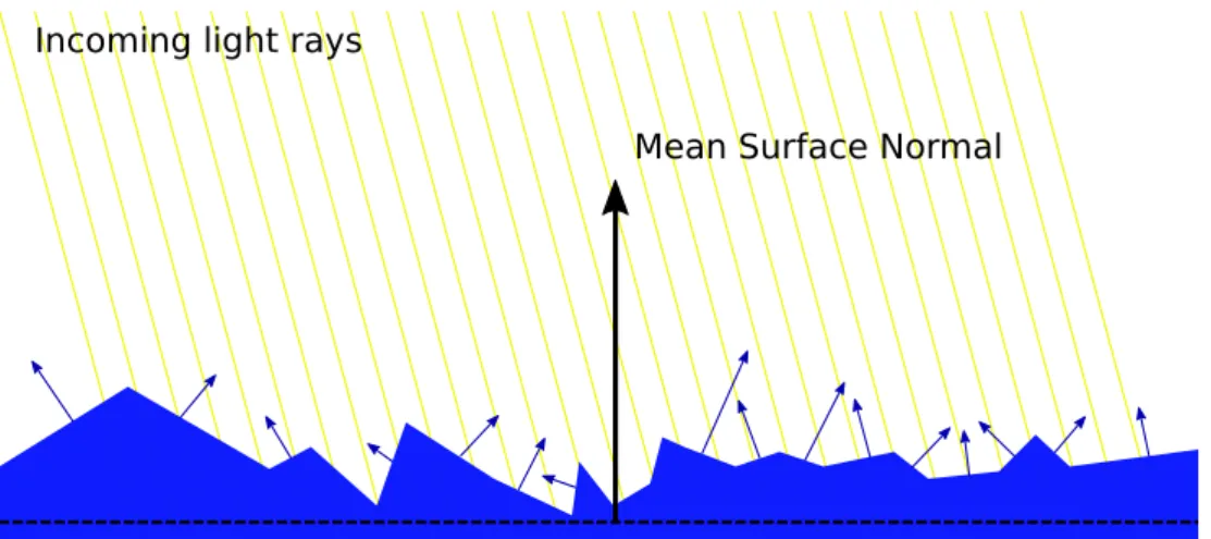
From here on many different BRDF models have been proposed, such as the Lommel-Seeliger model[55], which is interesting, because it explains why the Moon does not appear to be a Lambertian reflector. Other more physically cor-rect models build on the assumption of a microfacet model. The surface is mod-elled by randomly distributed micro reflectors, which act as tiny mirrors, see Fig-ure 2.4. A number of different models use this underlying microfacet model, for example the Torrance-Sparrow[58], Cook-Torrance[58], Ward[63], Oren-Nayar[41]

(31)

2.1 Light Transport

Figure 2.4: The microfacet model describes reflection properties by modeling a surface with randomly oriented microsurfaces. The underlying probability dis-tribution, as well as the roughness of the surface dominate the appearance of a surface.

and the Ashikhmin-Shirley model[3]. Exemplary the Cook-Torrance model is presented in a little more detail. The BRDF term for this model is given by

fr(ωi, ωo) =kd+ks

D(h₎_F₍ω_o₎_G₍ω_o_,ω_i₎

4(ω_o_·n₎₍n_·ω_i₎ , (2.11)

where D is the microfacet distribution, F the Fresnel factor and G the geomet-ric attenuation factor, which expresses the ratio of light which is occluded by other microfacets. The distribution term D controls how the microfacets are distributed, often a Gaussian distribution function is used. Another common function is the Beckmann distribution[6], given by

D(h_{) =} exp (−tan

2₍_α₎_/m2₎

πm2_cos4₍_α₎ , α= arccos(n·h), (2.12) wherem describes the roughness of the material. A larger roughness value leads

(32)

to a more diffuse appearance. The Fresnel factor describes how much of the inci-dent light is transmitted or reflected depending on the refraction indicesn1, n2 of the media at the interface. Additionally, the Fresnel equation takes into account polarization. We do not want to go into the details of the Fresnel equations, but just present the commonly used Schlick[53] approximation

F(θ) = F0+ (1−F0)(1−cosθ)5 (2.13) F0 = n 1−n2 n1+n2 2 , (2.14)

s where θ is the angle between the surface normal and the incident light ray. The geometric attenuation term expresses that neighboring parts can block of some light, that would otherwise reach a microfacet. This can be the case either when the light enters or exits the surface. Hence, it is given as

G= min 1,2(h·n)(ωo·n) ω_o_·h , 2(h_·n₎₍ω_i_·n₎ ω_o_·h ! . (2.15)

In practice these different models are often used combined to get realistic looking materials in computer graphics.

2.1.2 Light Model

Having all ingredients to describe the light interaction at a surface, the question remains how the flow of light in a complex scene can be described. Again, we

(33)

2.2 From Stereo to Light Fields

will point to ideas commonly used in computer graphics. The governing equation for the light transport is given by the render equation. It describes the amount of radiance emitted from a point in space xin direction ω_o _{of an observer. The}

amount of reflected light depends on the material properties, as discussed earlier. The incident angle of the light with respect to the surface normals is represented by the shading termn·wi and is heavily used in techniques such as shape from shading. The full equation is given by

L(x_,ω_o_{) =}_L_e₍ω_o_{) +}

Z

Ωfr(

ω_o_, ω_i₎_L₍ω_i_{) (}n_·ω_i₎_dω_i_, _(2.16)

where Le is an emission term, e.g. for a light source and Ω is the half sphere

around the surface normal. In practice it is impossible to find an analytical solution to this integral. This is due to the fact, that we need to take into account the incoming light contributions from all directions in the upper half sphere. The calculated radiance can then again contribute to the radiance of other points and depending on the geometry we have a complicated interaction scheme with a recursive definition. In computer graphics this problem can solved by ray tracing, where light rays are cast from an observer into the scene. Therefore, a Monte Carlo sampling method is used. The inverse process, the recovery of the light model parameters from several images is an even harder task, and mainly the goal of this thesis. But before introducing the techniques for recovering the BRDF and surface normals from multiple views, we will review the foundations of 3D reconstruction.

2.2 From Stereo to Light Fields

We will now present the theoretical foundation of 3D reconstruction in light fields. Before going into the details of light field imaging we recapture simple depth estimation via triangulation, which is the basis for stereo methods using only two views.

(34)

f f Right camera Left camera x b 3D point Image plane x_l xr

Figure 2.5: Scene geometry for estimating depth by triangulation. The different positions xl and xr for the projections of the 3D point x result in the disparity

d=xl−xr. The depth z can then be inferred by z = bf_d.

2.2.1 Stereo

When we image the same 3D scene from two different view points we have some constraints between these two projections. The underlying mathematical theory is the epipolar geometry. We assume rectified, calibrated images and a pinhole camera model. This means, that all epipolar lines are parallel to both image planes. Given two parallel, identical cameras we can infer the depth of a pointx

using the different positions in the image, under which this object appears, see Figure 2.5. This difference in location on the image sensor is called parallax or disparity d and relates to the depth z via

z = b·f

(35)

wheref is the focal length of the camera in px and the baseline b between the two camera projection centres. The greatest challenge is to actually find the same 3D point in both images. To do so, many methods rely on feature points, based on edges or corners. There is a whole family of these features, such as SIFT[34], SURF[5], ORB[47] and many others. In principal, all pixels have to be touched to find these feature points in the other image, which – with increasing image resolution – can be very time consuming, e.g. O(nm). Due to the rectification the search space can be constrained to the same epipolar lines, e.g. the same image row.

There are three major problems in finding good feature points, or to retrieve them.

Occlusionsappear when a 3D point is visible in one view, but not the other. For these points it is not possible to infer the depth via triangulation.

Featureless regions, such as blank walls, are difficult to handle as well. The lack of a significant feature prevents the correspondence search. Usually, interpolation methods are established to fill these regions.

Changing brightness for specular materials from one view to another can in principal be modelled and hence accounted for, but requires more information about the scene. This is the main focus of this thesis.

2.2.2 Light Fields

Instead of two views, light fields utilize many views to enhance the disparity estimation, see Figure 2.6. Stacking the same image row from each view on top of another we build a so called epipolar plane image (EPI), see Figure 2.7. The slopes of the resulting lines directly relate to the disparity between the different views.

(36)

3D Surface Point

Figure 2.6: To capture a structured light field, we add more cameras. For the ease of computation we keep the baseline between camera pairs constant.

A common parametrization for a light field is the so called Lumigraph [17, 30]. It is defined using two parallel planes Ω and Π. The first plane Ω addresses coordinates (x, y) ∈ Ω in the image domain . The second plane Π contains the focal points (s, t)∈Π of all cameras. The intensity for each pixel in each view is hence encoded in the light field

L: Ω×Π →R (s, t, x, y)7→L(s, t, x, y). (2.18)

To slice out an epipolar plane image (EPI), we fix the image dimension corre-sponding to the camera direction, i.e. for the horizontal direction we fixy =y∗

and t =t∗

(37)

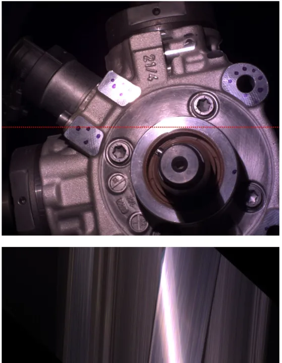
Figure 2.7: Object with a specular highlight. An epipolar plane image was built from different views and the same image row indicated by the red line. The EPI was reshifted for better visibility of the line structures.

(38)

St∗_,y∗(s, x) := L(s, t∗, x, y∗). (2.19)

The orientation in these EPIs directly encodes the disparity and hence the depth.

2.2.3 Structure Tensor

A very interesting opportunity arises now. Instead of searching for similar fea-tures among the different views, we can directly compute the local orientation in the EPI. One common used operator for orientation estimation is the structure tensorSwhich relates a tensor based on the partial image gradientsIx,Iy to each

pixel p, e.g. S(p) =    (Ix(p))2 Ix(p)Iy(p) Ix(p)Iy(p) (Iy(p))2   =:    Jxx Jxy Jxy Jyy   , (2.20)

where the partial gradients are usually a result of a convolution with one of the common edge detection filters, e.g. Sobel or Scharr, where the latter provides a better rotational symmetry. The disparity is then given by

d= tan 1 2arctan 2Jxy Jxx−Jyy !! , (2.21)

(39)

Additionally, a confidence measure called the coherence c ∈ [0,1] [8] can be calculated by c= v u u t (Jxx −Jyy)2+ 4(Jxy)2 (Jxx+Jyy)2 , (2.22)

where c = 1 relates to a sharp orientation in a specific orientation and c = 0 relates to a uniform region where no clear orientation is visible.

2.2.4 Hough Transform

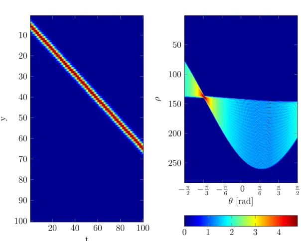
Besides, estimating the orientation only locally, also global methods, which take the whole EPI information into account are available. The Hough Transform is a widely known method which maps image features, such as lines or circles, to a parameter space, see Figure 2.8. Lines, circles or other parameterizable shapes become then easily identifiable in the parameter space. However, this comes at a great computationally cost, since al possible parameters must be traversed. Additionally, the classical Hough transform suffers from the implicit discretization in the parameter space. To reduce computational overhead and address the discretization issue, random sampling methods are of great use and referred to as probabilistic Hough transform [57, 27].

(40)

−π 2 − π 3 − π 6 0 π 6 π 3 π 2 50 100 150 200 250 θ [rad] ρ 0 1 2 3 4 20 40 60 80 100 10 20 30 40 50 60 70 80 90 100 t y

Figure 2.8: Representation of a straight line in Hough space in the y t-plane. On the left hand side the line in image space is visualized. The right hand side shows the corresponding hough transformation with intensity values on a logarithmic scale. Image taken from [19].

(41)

3

Capturing the Light Field

The following chapter deals with the aspects of capturing light field data, espe-cially in combination with specular highlights. Part of it emerged in collaboration with Bosch to develop an understanding of the challenges of light field capture for specular highlights. The first part deals with different hardware setups to cap-ture a light field. The second analyses specific trajectories to probe a sufficient part of the object to reconstruct the BRDF.

Especially for light field capturing a precise camera calibration is necessary. For this thesis we used fractal calibration targets to get robust results, especially at the image edges [51].

3.1 Capturing Devices

In the following, different measurement techniques to capture a light field are presented.

(42)

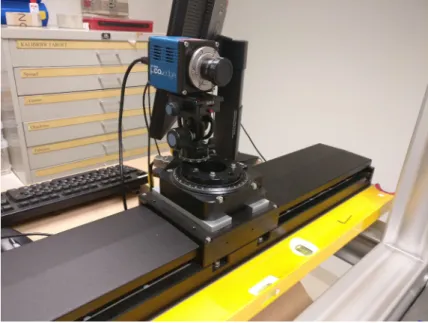
Figure 3.1: Light fields can be captured using a translation stage with a mounted camera. This is a cost-effective setup, but only static scenes can be captured.

3.1.1 Translation Stage

A camera can be mounted on a movable platform, also known as translation stage. The accuracy is in the order of micrometers for translation ranges of up to a meter. An example for a linear translation stage can be seen in Figure 3.1. The need for only a single camera makes it cost efficient, and easier to calibrate since the intrinsic parameters do not change from view to view. Dynamic scenes can not be captured. Special care must be taken to prevent changing illumination, which would negatively affect the analysis of the material properties.

3.1.2 Camera Array

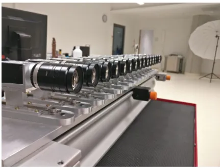
In contrast to a translation stage a camera array consists of multiple cameras which have a fixed relation to each other. This way, it is possible to capture dynamic scenes. Here precise calibration between the cameras is critical. An

(43)

3.1 Capturing Devices

Figure 3.2: With a linear camera array in a verged setup also dynamic scenes can be captured.

technical hurdle is the synchronized capture and the storage of the often enormous amounts of data in parallel. A linear camera array is displayed in Figure 3.2, where the cameras are verged to one focal point.

3.1.3 Microlens Arrays

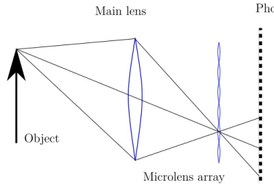
A third option, not used in this thesis, are microlens arrays in front of a single image sensor, see Figure 3.3. Each photon is redirected to a different set of pixels on the sensor depending on its direction. The direction of the light ray can be inferred by the position on the pixel grid. The advantage is the low cost, but it suffers from a small baseline and a greatly reduced effective resolution. Nonetheless, this technique made its way into the consumer market, where the user can profit from certain light field applications, such as refocusing. Precise 3D reconstruction is not achievable, due to the small baseline. Recently ideas have emerged to use transparent photo-detectors based on graphene [40] to capture

(44)

Object

Main lens

Microlens array

Photosensor

Figure 3.3: Consumer cameras such as the Lytro use a microlens array to capture a light field. Proportions are not to scale.

a light field. This would circumvent the inherent trade-off between image and angular resolutions for single sensor platforms.

3.2 Optimal Trajectories through the BRDF Space

An optimal acquisition setup should make it possible to acquire as much infor-mation about the surface properties as possible. The diffuse part is not changing much from view to view, so the most interesting changes are happening close to the specular lobe. In the following we will discuss how we can ascertain that a large portion in the light field contains information relevant for BRDF extraction.

(45)

3.2 Optimal Trajectories through the BRDF Space

n _r

l

v1 vn

p0

Figure 3.4: The surface normal range which can be recovered by a light field setup is limited by the geometry between camerasv1,v2, ...,vn, object and light source.

3.2.1 Geometric Consideration of the Camera Setup

Before we go into details about optimality we want to answer the simple question which surface normal range can be, in principle, recovered from a light field setup. Let us assume a linear light field setup withncameras and a baselineb therefore spanning a distance of Ds = nb. A point of a specular surface of interest may be at the location p0 and a point light source at the position L, see Figure 3.4.

(46)

Assuming perfect reflection, a light ray l will be reflected into the direction r

according to

r=l−2(l·n)n, (3.1)

where n is the surface normal. To capture the maximum of the specular part, r

must reside withinv1 and vn. Otherwise, we still can see some part of the lobe, but the exact reconstruction becomes more difficult as we can see in chapter 4.

3.2.2 Half-way Vector Parametrization

There are several remarks which highlight the most important implications: We can expect specular reflection if the surface normal and the half vector are aligned (Θh = 0). For isotropic BRDFs we have no dependence on Φh, reducing the

BRDF to three dimensions. Viewing 2D slices along the Φddirection yields, that

most information is contained at Φd = π₂ and the other slices look like similar

versions with some parts excluded. Another interesting characteristic is that the specular reflection varies mostly along the Θh axis and less so along the other

axes. In Figure 3.5 a subspace of BRDF from three different materials is shown. By capturing light fields with a single moving camera we essentially cut out trajectories from the BRDF subspace. The trajectory depends on the camera path and the position of the light source. A desirable path would move in the 2D BRDF slice along the Θh dimension with a small and constant Θd, to guarantee

(47)

Gold paint Blue phenolic Aluminium oxide

Figure 3.5: Inspecting 2D slices of BRDFs in half-way vector space we can see how the characteristics of different materials differ. For example the fall off rate for aluminum oxide is much larger than for gold paint. The data is scaled logarithmically for better visibility and taken from the MERL database[36].

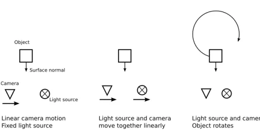
Linear camera motion Fixed light source

Light source and camera move together linearly

Light source and camera ﬁxed

Object rotates

Object

Surface normal Camera

Light source

(48)

3.2.3 Linear Camera Motion and Fixed Light Position

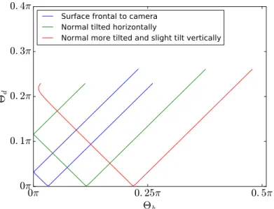
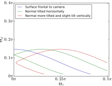
To illustrate the importance of knowing the surface normal to estimate the BRDF of a given object we will investigate the trajectories through the 2D BRDF space defined by the two angles in half-way vector parametrization. In Figure 3.7 we see different trajectories based on various normal orientations for an acquisition setup where the camera is moving linearly. If we recall that the specular area of the BRDF runs along the Θd-axis, we notice that the red trajectory – where

the surface normal is slightly out of the plane spanned by the object point, the camera and the light source – does not touch the y-axis, effectively resulting in a reduced peak width in the corresponding 1D-BRDF slice taken from the EPI.

0π 0. 25π 0. 5π Θh 0π 0. 1π 0. 2π 0. 3π 0. 4π Θd

Surface frontal to camera Normal tilted horizontally

Normal more tilted and slight tilt vertically

Figure 3.7: Trajectories through the 2D BRDF space for a straight moving camera and a fixed light source. The camera moves in the x direction perpendicular to its viewing direction anti-parallel to the surface normal (in the blue case). The green trajectory describes a path were the surface normal is tilted by 22◦

around the y-axis (pointing upwards). The red trajectory is tilted by 45◦ _{around the}

(49)

3.2.4 Linear Camera Motion and a Co-Moving Light Source

For the case of a moving light source, depicted in Figure 3.8, we see that the trajectory through the 2D BRDF slice crosses a much narrower part along the Θdaxis than in the case of a fixed light source. That the trajectory is still crossing

along the Θdaxis stems from the fact, that the distance between the camera and

light source pair and the object point is changing and therefore the difference angle increases with decreasing distance to the object point. Basically, the larger the distance between light source and camera, the greater is the coverage in the Θd direction. This effect could be suppressed entirely using a confocal setup,

where the light source and the camera are basically at the same position. This would open up the possibility to use only 1D BRDF slices, since we would set Θd to zero. 0π 0. 25π 0. 5π Θh 0π 0. 1π 0. 2π 0. 3π 0. 4π Θd

Surface frontal to camera Normal tilted horizontally

Normal more tilted and slight tilt vertically

Figure 3.8: Trajectories through the 2D BRDF space for a straight moving cam-era and a co-moving light source. The different colors encode the same normal displacements as in Figure 3.7.

(50)

3.2.5 Fixed Camera and Light Source, Rotating Object

In Figure 3.9 we the the BRDF trajectories for an object describing a circular motion in front of the camera. The extension along the Θd axis is much smaller

than previous cases. Again the BRDF trajectory for the slightly vertical tilted normal is not reaching Θh = 0.

0π 0. 25π 0. 5π Θh 0π 0. 1π 0. 2π 0. 3π 0. 4π Θd

Surface frontal to camera, d = 1 Normal tilted horizontally, d = 5

Normal more tilted and slight tilt vertically, d = 20

Figure 3.9: Trajectories for circular motion. The distance between camera and light source is given by d.

3.2.6 Optimal Acquisition

To capture all of the BRDF information multiple combinations of light source and camera position must be probed. A possible implementation would involve a circular light field with a fixed light source. To probe along the Θd-axis, the light

position must be varied, e.g. in a circular fashion around the object. Figure 3.10 shows a resulting BRDF coverage by such a setup. It must be noted that surface

(51)

3.2 Optimal Trajectories through the BRDF Space 0π 0.1π 0.2π 0.3π 0.4π 0.5π Θh 0π 0.1π 0.2π 0.3π 0.4π 0.5π Θd

BRDF Cover for a Circular Light Field with varying Light Position

0.0 0.1 0.2 0.3 0.4 0.5 0.6 0.7 0.8 0.9 1.0

Figure 3.10: BRDF coverage of a circular light field with different light positions. Differently colored lines encode the light position. The light position is also varied in a circular fashion around the object. Zero indicates the start position close to the camera and one the opposite site of the circle. The camera is stationary and the surface normal is in the same plane spanned by the light source and camera. normals which lie not in the same plane as the camera and the light source will not fully reach the Θd-axis and therefore have reduced intensities. To address this

challenge the object needs to turn around an additional axis. Basically, what we have then is a goniometer. To limit the search area to the high intensity regions of the specular peak and the Fresnel effect, two light positions are sufficient. The first one very close to the camera and the second in opposite direction, to capture the Fresnel contribution.

(52)

(53)

4

Surface Normal Estimation via

Geometrical Optics

In this chapter we will discuss a method to extract surface normals from specular highlights for glossy materials. We assume a given depth and illumination. We make no assumptions about the shape of the BRDF but instead focus on the highlight position.

4.1 The Inverse Problem

Reconstructing the geometry, light source and material properties is way more challenging than the forward process, where everything is known and images can easily be rendered. This becomes especially evident when considering how many different combinations of materials, textures, geometries and lightning conditions could lead to the same image. This intrinsic ambiguity is difficult to resolve and human brains have a broad collection of heuristics to deal with it, even if they close one eye, and stay still, and do not defocus.

Using two or more images allows us, with some assumptions, to use triangu-lation to infer the depth of a scene as explained in section 2.2. The assumption of brightness constancy, which only holds for Lambertian surfaces, is in reality

(54)

Figure 4.1: EPI with specular highlight.

often violated. Triangulation entirely fails if a point in 3D space is only visible in one image. This leads to a tricky trade-off, especially in stereo vision, where a large base line leads to higher accuracy but also to more occluded areas.

Here light fields provide a nice best-of-all solution, since they can cover a large base line to give better accuracy but also provide information in between to reduce occlusions. They also offer a possibility to reconstruct non Lambertian surfaces. Specular highlights appear almost everywhere in real life and are due to the microscopic structure of physical objects. As explained in section 2.1, diffuse materials have a random distribution of mircofacets around the surface normal and hence appear the same from different vantage points. If this distribution favors a direction, we see a highlight when the viewing direction aligns with the resulting reflectance angle. Here, standard 3D reconstruction algorithms based on the brightness constancy start to break down. A bright pixel in one view appears less intense in another. Without any further assumptions about the reflectance properties the only way to handle this missing correspondence, is to use neighbouring regions where correspondences have been found.

In the EPI, see Figure 4.1, we can observe the gradual intensity change from one view to another.

(55)

4.2 Solving the Inverse Problem by Geometry l r v Diffuse Reflection Specular Reflection Camera Direction 2 Camera Direction 2 Surface Point Light Source

Figure 4.2: Sketch of the cross array setup. q1 and q2 are the nearest points to

r_{. Hence, in the closest view we will see an intensity maximum.}

4.2 Solving the Inverse Problem by Geometry

The surface normaln can be calculated if the direction of the light sourcel _and

the direction of reflectionr _{is known}

n = r+l

kr₊l_k. (4.1)

Unfortunately, we do not know neither the direction of reflection r _{nor the}

surface normaln. All we have are our different camera positionsωo and intensity maxima along each direction of our cross setup which we can relate to a 3D point

(56)

1. The intensity is highest in the direction of the reflection.

2. The decrease in intensity away from the reflection ray is rotationally sym-metric.

Using these assumptions we can infer from two intensity maximum positions the direction of reflection r_. _{We suppose that} _ω_i _{as well as our 3D surface point}

p0 is known. The camera centres lie on two independent lines with directions

g1 = (1,0,0)T and g2 = (0,1,0)T and a support point at (0,0,0)T.

When observing a specular peak along g1 and g2, we eventually spot a maxi-mum in intensity in the view closest toq1 and q2, see Figure 4.2. If we presume isotropic reflection, meaning that the intensity lobe has a rotational symmetry around r_{, we can conclude that the points} _q₁ _and _q₂ _{have minimal distance}

to the yet unknown r_{. This leads to an interesting geometric problem, where}

we want to solve for r _{and hence for the surface normal} _n_{. This can be solved}

analytically, but leads to a very long unusable expression (see section A.1 for details). Thus, we formulate this as an optimization problem. For a given re-flection vector we expect the specular highlights at certain points in our camera geometry. Hence we minimize the difference of these proposed highlight positions q′

i to the measured positions qi. The objective function f is then given by

argmin q′ i f =X i (qi−qi′)2. (4.2)

We do not limit ourselves to only two independent directions, since we can have, at least in theory, arbitrary many. The q′

i are calculated by q′ i =pi+ (p0−pi)·s gi·s gi (4.3)

(57)

4.3 Results

with

s=r_×₍gi×r). (4.4)

and pi is the support vector for the camera directions which is in general set to zero for all i. For two independent directions of observers the solution is unique up to the magnitude of the direction vector of r_.

4.3 Results

To quantify the effects of noise in the image signal and the number of cameras the intensity distribution for a single 3D point was simulated. The intensity distribution is generated with a Blinn-Phong model with the parameters kd =

10.0, ks = 10000.0 and m = 3.0. The geometry is given by a single 3D point

at (0,0,−10)T_{, a point light source at (0}_,₀_,₀₎T _{and a camera cross setup with}

a distance of 50 between the most left and most right camera, all in arbitrary units. We randomly draw 100 surface normals with an angle up to 45◦

with respect to the virtual camera ray. In one experiment we take a fixed number of 17 cameras per view direction and increase the relative noise from 10−4 _{up to} 102_{, see Figure 4.3. The angular error remains below 4}◦ _{up to a relative noise}

of 0.01 and increases then up to 17◦ _{for a relative noise of 4}_._{0. This limit is due}

to the initial range of possible surface normals, where by rare chance it is very unlikely to produce an angle error larger than 20◦

.

In Figure 4.4 a similar experiment was carried out. Instead of increasing the noise, the noise is kept constant to 0.05 of the intensity signal and the number of cameras used is increased. The decrease of the angular error is to be ex-pected, since errors here result mostly from the insufficient angular sampling of the cameras. By adding more and more cameras the error goes down up to one degree.

(58)

In principal we can calculate the surface normal in a simple an efficient fashion, but we face three major practical issues:

1. At least two peaks must be visible. If one of the peaks is outside the visible range we need to extrapolate, which will likely lead to poor results.

2. The result suffers angular discretization depending on the number of views. This can be avoided by using an interpolation method. This directly leads to questions about how to model intensity distributions in light fields and is tackled in section 5.1.

3. Due to the unique solution we can not evaluate the "goodness" of the ap-proximation.

To circumvent all these issues we will derive a method which includes all in-tensity values from all views by applying an appropriate reflection model. None the less it provides a fast method for deriving the surface normal components if specular highlights are visible.

(59)

4.3 Results

Figure 4.3: Accuracy depending on the relative signal noise. The error-bars represent the standard deviation given by σ=

r PN

i=1(xi−x)2

N−1 . The angular error does not approach zero due to quantization of the highlight position by the fixed number of cameras.

(60)

(61)

5

Simultaneous BRDF and Surface

Normal Extraction

The following chapter has been published in part in [20]. Additional results are highlighted if they appear in the thesis for the first time.

5.1 Solving the Inverse Problem using a BRDF

Model

As seen in chapter 4, we can infer surface normals using the maxima of two linearly independent camera directions. While this is already useful if both di-rections include the reflection lobe, we are at a loss if this is not the case. To infer normals, even when the reflection peak is outside the viewing geometry, we use not only the position of the maximum, but the full intensity distribution. The intensity variation along one viewing direction constrains the surface normal in one dimension. Therefore, we use an orthogonal second direction, which is given by a cross-shaped camera array, to constrain the surface normal in two dimen-sions. In our approach we use the intensity distribution as observed from both acquisition directions. We can picture the different intensity distributions as cuts through the 3D specular lobe. This means that we can still deliver estimates,

(62)

even if only a part of the specular lobe is visible.

Recalling chapter 2, we can model the incoming intensity from a point x by

L(x, ωo) =Le(ωo) +

Z

Ωfr(n, ωo, ωi)L(ωi) (n·ωi)dωi. (2.16 rev.)

There are two major challenges in solving this equation. Firstly, we need to integrate over all incoming light directions, and hence need to know the incoming radiation for all points. Secondly, light bounces of each surface, leading to a complicated interaction between active light sources, reflecting surfaces and the geometric relation between them. While the first challenge could be tackled by capturing the light using a dome, multiple light bounces are very difficult to resolve inversely. To simplify the problem we assume single light bounces and dominant light sources. We separate the incoming light dependency into a dominant term Ld and a perturbation termLp

L=Ld+Lp, (5.1)

where we assume, that the perturbation is negligible.

Assuming a discrete number N of dominant incoming light directions and assuming single light bounces we yield

Ld= N

X

j=1

(63)

5.1 Solving the Inverse Problem using a BRDF Model In ten sity Observer Position Observer Position Image P os ition Data Model

Figure 5.1: An intensity distribution can be obtained using the disparity in the EPI. Given a correct disparity, the intensity distribution depends on the relative orientation of the surface, the material properties and the illumination.

(64)

This leads to a nonlinear regression problem in the form of argmin Θ,n f = M X x=1 kLd(Θ,n, ωo,x)−I(ωo,x)k, (5.3)

whereΘare the BRDF parameters and I(ωo,x) is the measured intensity for the

3D point in the x-th view, consideringM different views.

Using traditional solving schemes, such as the Levenberg-Marquardt algorithm, we need to provide parameter initializations which allow for a successful conver-gence. For the BRDF parameter these depend on the width and relative height of the peak, see Figure 5.1. A good initialization for the surface normal is given by

ninit =

wi+wo,x

kwi+wo,xk

, (5.4)

where the x-th optical system is usually in the center of the cross setup. As can been seen from the form of objective function, minimization can be trapped in a local minimum, see Figure 5.3. To make the convergence more robust, we restart the optimization with random normals, in case the residual is above a certain threshold. The surface normals are very accurate as can be seen in subsection 5.3.3, but we have to keep in mind that we assume the 3D point a priori, which is in general not given. Especially for regions where specular reflection occurs the reconstruction of the geometry is very difficult. So this method can only be applied if the geometry is known beforehand, e.g. by using a CAD model of the object of interest. Therefore, the next chapter deals with estimating also the disparity simultaneously.

(65)

5.2 Implementation for Real and Synthetic Light Field Data

Figure 5.2: Process of simultaneously estimating surface normals and BRDF parameters.

5.2 Implementation for Real and Synthetic Light

Field Data

The processing pipeline is depicted in Figure 5.2. As input the method requires the calibrated camera and light source positions, as well as approximate depth estimates. To calculate an initial disparity map we use the structure tensor method proposed by Wanneret al. [61].

EPIs encode, besides the depth information, also the intensity distribution, along each orientation line, needed to determine material properties.

Regarding the surface points visible in the center view, we use the disparity, to map the input intensities to an image stackL′

(k, x, y) whereL′

x∗_,y∗(k) represents the intensity distribution for a single surface point as observed from different views, see subsection 5.2.1. A second stack is generated accordingly using the disparity as input data. This way, occlusion maps can be computed easily, as detailed in subsection 5.2.2. They prevent the algorithm from mixing foreground and background information. By regarding the unoccluded intensity values, we can identify surface points which exhibit specular characteristics by measuring the intensity change along the views, see subsection 5.2.3.

Finally, we optimize the BRDF parameters and the surface normal indepen-dently for each pixel, for the regions where we identified specular intensity vari-ations, see subsection 5.2.5. Our method works on the following assumptions:

(66)

• We assume an approximate disparity map, in our implementation we utilize the structure tensor.

• The cameras, as well as the light source is calibrated in terms of location and camera intrinsics.

• The light transport is dominated by the single-bounce reflection of a point light source.

• At least two independent viewing directions are needed, e.g. by using a cross setup.

5.2.1 Preprocessing

To compute the intensity changes of object points in an efficient manner, we need to address all pixels related to a specific surface point. This principle is similar to the reshifting in EPI processing as introduced by Diebold and Goldluecke [12]. The specific shifting is given for the horizontal light field by s

I′

(k, x, y) =I(k, x+d·(c−k), y), (5.5) which maps all related pixels to a vertical line, which is easy to access for further processing, see Figure 5.4. The variablec corresponds to the index of the center view and d to the disparity of the center view at (x, y). The vertical viewing direction is handled analogously. It is important to note here, that the method is especially well suited to smooth, texture-less regions. Here, erroneous dispar-ities have a low impact on the accuracy of the normal estimation, since even if intensity information from neighbouring surface points are mistakenly used, the material properties change slowly compared to the error in the disparity. These areas are particularly difficult for conventional methods, which rely on structural information, such as strong image gradients. This way we can utilize even

Light Fields Reconstructing Geometry and Reflectance Properties

Dissertation

submitted to the

Combined Faculties for the

Natural Sciences and for Mathematics

of the Ruperto-Carola University of Heidelberg, Germany

for the degree of

Doctor of Natural Sciences

put forward by

M.Sc. Marcel Gutsche

born in Frankfurt am Main, Germany

Date of oral exam: July, 16th 2018

Light Fields

Reconstructing Geometry and

Reflectance Properties

PD Dr. rer. nat. Christoph Garbe

Prof. Dr. rer. nat. Karl-Heinz Brenner

Acknowledgements

Contents

1

Introduction

1.1 Motivation

1.2 Related Work

1.3 Contribution

1.4 Outline

2

Theory of Light Fields and

Reflectance

2.1 Light Transport

Re

ﬂ

ection

Surface

Absorption

Transmission

2.1.1 The Bidirectional Reflectance Distribution Function

2.1.2 Light Model

2.2 From Stereo to Light Fields

2.2.1 Stereo

2.2.2 Light Fields

2.2.3 Structure Tensor

2.2.4 Hough Transform

3

Capturing the Light Field

3.1 Capturing Devices

3.1.1 Translation Stage

3.1.2 Camera Array

3.1.3 Microlens Arrays

3.2 Optimal Trajectories through the BRDF Space

3.2.1 Geometric Consideration of the Camera Setup

3.2.2 Half-way Vector Parametrization

3.2.3 Linear Camera Motion and Fixed Light Position

3.2.4 Linear Camera Motion and a Co-Moving Light Source

3.2.5 Fixed Camera and Light Source, Rotating Object

3.2.6 Optimal Acquisition

4

Surface Normal Estimation via

Geometrical Optics

4.1 The Inverse Problem

4.2 Solving the Inverse Problem by Geometry

4.3 Results

5

Simultaneous BRDF and Surface

Normal Extraction

5.1 Solving the Inverse Problem using a BRDF

Model

5.2 Implementation for Real and Synthetic Light

Field Data

5.2.1 Preprocessing