A Particle Swarm Optimization based Optimal Power
Flow Problem for Iraqi Extra High Voltage Grid
Firas M. Tuaimah
University of BaghdadBaghdad, Iraq
Montather F. Meteb
University of Baghdad Najaf, Iraq
ABSTRACT
The objective of an Optimal Power Flow (OPF) algorithm is to find steady state operation point which minimizes generation cost, loss, load ability etc. while maintaining an acceptable system performance in terms of limits on generators real and reactive powers, line flow limits etc. The OPF solution includes an objective function. A common objective function concerns the active power generation cost. A Particle Swarm Optimization is proposed to solve the OPF problem. The Particle Swarm Optimization (PSO) is used to minimize the generating cost as an objective function through the inequality constraints as well as the conventional load flow is used to perform the equality constraints. A computer program, written in MATLAB environment, is developed to represent the proposed method. The adopted program is applied for the first time to Iraqi 24 bus Super High Voltage (SHV) network (400 kV). The required are data taken from the Iraqi National Control Center (INCC), which belongs to the ministry of electricity.
Keywords
Optimal power flow, Particle Swarm optimization (PSO), active power dispatch.
1. INTRODUCTION
Throughout the entire world, the electric power industry has undergone a considerable change in the past decade, and
will continue to do so for the next several decades. In the past, the electric power industry has been either a government-controlled or a government-regulated Industry which existed as a monopoly in its service region. All people, businesses, and industries were required to purchase their power from the local monopolistic power company. This was not only a legal requirement, but a physical engineering requirement as well. It just did not appear feasible to duplicate the resources required to connect everyone to the power grid. Over the past decade, however, countries have begun to split up these monopolies in favor of the free market [1]-[3].
Optimal Power Flow (OPF) solution methods have been developed over the years to meet this very practical requirement of power system operation [4]-[7].
The optimal power flow problem has been discussed since its introduction by Carpentier [8]. Because the OPF is a very large, non-linear mathematical programming problem, it has taken decades to develop efficient algorithms for its solution. Many different mathematical techniques have been employed for its solution. The majority of the techniques discussed in the literature use one of the following five methods [9]-[12]: 1. Lambda iteration method, also called the equal incremental cost criterion (EICC) method.
2. Gradient method. 3. Newton’s method.
4. Linear programming method. 5. Interior point method.
Newly developed heuristic approaches called particle swarm optimization (PSO) has been introduced. This method combines social psychology principles and evolutionary computation to motivate the behavior of organisms such as fish schooling, bird flocking, etc.
Particle swarm optimization, abbreviated as PSO, is based on the behavior of a colony or swarm of insects, such as ants, termites, bees, and wasps; a flock of birds; or a school of fish. The particle swarm optimization algorithm mimics the behavior of these social organisms. The word particle denotes, for example, a bee in a colony or a bird in a flock. Each individual or particle in a swarm behaves in a distributed way using its own intelligence and the collective or group intelligence of the swarm. As such, if one particle discovers a good path to food, the rest of the swarm will also be able to follow the good path instantly even if their location is far away in the swarm. Optimization methods based on swarm intelligence are called behaviorally inspired algorithms as opposed to the genetic algorithms, which are called evolution-based procedures. The PSO algorithm was originally proposed by Kennedy and Eberhart in 1995 [13].
In the context of multivariable optimization, the swarm is assumed to be of specified or fixed size with each particle located initially at random locations in the multidimensional design space. Each particle is assumed to have two characteristics: a position and a velocity. Each particle wanders around in the design space and remembers the best position (in terms of the food source or objective function value) it has discovered. The particles communicate information or good positions to each other and adjust their individual positions and velocities based on the information received on the good positions[14].
This paper presents a Particle Swarm Optimization -based Optimal Power Flow for generation cost minimization using as control variable the generator active power. The PSO based OPF proposed in this paper improves the accuracy of the convergence of an objective function.The proposed approach has been examined and tested on Iraqi Super High Voltage (SHV) grid. The potential and effectiveness of the proposed approach are demonstrated. Additionally, the results are compared to Linear Programming (LP) method.
2. PROBLEM FORMULATION
The objective function contains real power generation cost. Mathematically, it is formulated as follows:
F = (1) Subject to
≤ ij ∊ (3) ≤ ≤ i ∊ (4) Where
P D : The real power load
: The power flow of transmission line ij
: The power limits of transmission line ij : The network losses
: The cost function of the generator i
: The number of transmission lines : The number of loads
The real power flow equation of a branch can be written as follows[15]:
= − ( cos + sin ) (5)
The bus power injection equation can be written as
= (6)
Where
: The sending end real power on transmission branch ij : The node voltage magnitude of node i
: The difference of node voltage angles between the sending end and receiving end of the line ij
: The susceptance of transmission branch ij
: The conductance of transmission branch ij
3. BASIC ELEMENTS OF THE PSO
TECH-NIQUE
The basic elements of PSO technique are briefly stated and defined as follows:
Particle, : It is a candidate solution represented by an m-dimensional vector, where m is the number of optimized parameters. At time i, the jth particle can be described as
= [ , ..., ],where xs are the optimized parameters and is the position of the jth particle with respect to the kth dimension, i.e. the value of the kth optimized parameter in the jth candidate solution.
Population, pop(t) : It is a set of n particles at time i, i.e. pop(i) = [ , ..., ]T.
The number of particles in population between (20 to 30). Swarm: It is an apparently disorganized population of
moving particles that tend to cluster together while each particle seems to be moving in a random direction[16]. Particle velocity, : It is the velocity of the moving
particles represented by an m-dimensional vector. At time i, the jth particle velocity can be described as = [ , ..., ],where is the velocity component of the jth particle with respect to the kth dimension.
Inertia weight, : It is a control parameter that is used to control the impact of the previous velocities on the current velocity. Hence, it influences the trade-off between the global and local exploration abilities of the particles[16]. For initial stages of the search process, large inertia weight to enhance the global exploration is recommended while, for last stages, the inertia weight is reduced for better local exploration.
Individual best, : As a particle moves through the search space, it compares its fitness value at the current position to the best fitness value it has ever attained at any time up to the current time. The best position that is associated with the best fitness encountered so far is called the individual best, . For each particle in the swarm, can be determined
and updated during the search. In a minimization problem with objective function f, the individual best of the jth particle is determined such that f( ) ≤ f( ) , e ≤ j . For simplicity, assume that f* = f( ). For the jth particle, individual best can be expressed as = [ , ..., ]. Global best, : It is the best position among all individual
best positions achieved so far. Hence, the global best can be determined such that f ( ) ≤ f ( ), j=1……,n . for
simplicity, assume that, f** = f ( ) .
Stopping criteria: these are the conditions under which the search process will terminate. The search will terminate if one of the following criteria is satisfied : (a) the number of iterations since the last change of the best solution is greater than a pre-specified number or (b) the number of iterations reaches the maximum allowable number [2&5].
4. COMPUTATIONAL
IMPLEMENTATIO-N OF PSO
The computational flow of PSO technique can be described in the following steps:
Step 1 ( Number of Particles) :
Assume the size of the swarm (number of particles) is N. To reduce the total number of function evaluations needed to find a solution, we must assume a smaller size of the swarm. But with too small a swarm size it is likely to take
longer to find a solution or, in some cases, it may not be able to find a solution at all. Usually a size of 20 to 30 particles is assumed for the swarm as compromise.
Step 2 (Initial position) :
Generate the initial population of X in the range and randomly as , , . . . , . Hereafter, for convenience, the particle (position of) j and its velocity in iteration i are denoted as and , respectively. Thus the particles generated initially are denoted , , . . . , . The vectors (j = 1, 2, . . . ,N) are called particles or vectors of coordinates of particles(similar to chromosomes in genetic algorithms).
Step 3 (Initial velocity) :
Find the velocities of particles. All particles will be moving to the optimal point with a velocity. Initially, all particle velocities are assumed to be zero.
Step 4 (Set local and global best positions)
Each particle in the initial population is evaluated using the objective function, f. For each particle, set = and
= , j = 1,...,n. Search for the best value of the objective function Set the particle associated with as the global best, ,with an objective function of . Set the initial value of the inertia weight w(0).
Step 5 (Updating the Iteration)
Update the iteration number as i = i + 1.
Step 6 (Weight updating): Update the inertia weight
= - ( ) * i
Step 7 (velocity updating):
= + c1 r1 ( - ) +c2r2 ( - ) (7) where c1 and c2 are positive constants and r1 and r2 are
uniformly distributed random numbers in [0,1]. It is worth mentioning that the second term represents the cognitive part of PSO where the particle changes its velocity based on its own thinking and memory. The third term represents the social part of PSO where the particle changes its velocity based on the social-psychological adaptation of knowledge. If a particle violates the velocity limits, set its velocity equal to the limit.
Step 8 (Position updating):
Based on the updated velocities, each particle changes its position according to the following equation:
= + (8)
If a particle violates its position limits in any dimension, set its position at the proper limit.
Step 9 (individual best updating):
Each particle is evaluated according to its updated position. If, < j=1,…….,N
then update individual best as : = and =
and go to step 10; else go to step 10.
Step 10 (Global best updating):
Search for the minimum value among , where min is the index of the particle with minimum objective function. If <
then update global best
= and = and go to step 11; else go to step 11.
Step 11 (Stopping criteria)
If one of the stopping criteria is satisfied then stop; else go to step5.
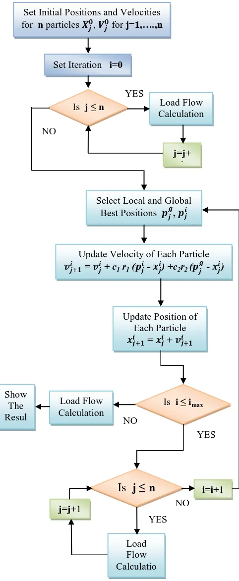
Figure 1. shows the flowchart of optimal power flow using particle swarm optimization.
5. CASE STUDY
The Iraqi 400kV (SHV) network was chosen to implement the proposed PSO algorithm for OPF.
The Iraqi SHV network consists of 24 Bus-bars, 38 transmission lines and 11 generating stations. Two operational case studies for the Iraqi network were chosen to be studied by this paper for optimal power flow solution. These two case studies are with cheap and expensive international fuel price conditions.
[image:3.595.319.560.70.656.2]All the data for this work was taken from the Iraqi National Control Center (INCC) that belongs to the ministry of electricity.
Table 1 indicates transmission system parameters in p.u. / km (at a base of 100 MVA) for the three types of the transmission lines used in the Iraqi network.
Figure 1. Flowchart of optimal power flow using particle swarm optimization
YES
NO
NO
YES
NO
YES Set Initial Positions and Velocities for n particles , for j=1,….,n
Set Iteration i=0
Is j ≤ n Load Flow
Calculation
j=j+
1
Select Local and Global Best Positions ,
Load Flow Calculation Show
The Resul ts
Is i ≤ imax
Update Velocity of Each Particle
= + c1 r1 ( - ) +c2r2 ( - )
Update Position of Each Particle
= +
Is
j ≤ n
i=i+1Load Flow Calculatio
n
Table 1 Iraqi transmission line system parameter
Conductor Type
R p.u. / km
X p.u. / km
B p.u. / km
AAAC 0.00002167 0.000197 0.005837
ACSS 0.0000228 0.0001868 0.005784
ACSD 0.0000228 0.0001897 0.005962
6. RESULTS
[image:4.595.316.554.89.281.2]The algorithm described in this paper has been coded in MATLAB (R2008a) language. The performance of the algorithm is illustrated considering for a state of load of the operation of the Iraqi power system. The results obtained from using Particle Swarm Optimization (PSO) method are compared with the results obtained from optimal power flow using Linear Programming (LP) method. There are four power plants run on two types of fuel to generate electric power, so we compared the results when they operate on the cheap fuel type and expensive fuel type. Figure 2. shows the voltage magnitude in per unit for each bus when cheap fuel price is used to generate power in power plants that operate on two types of fuel and for the two algorithms (Linear Programming and Particle Swarm Optimization).
Figure 2. Voltage magnitude at each bus with cheap fuel price
Figure 3. shows the generation of each plant for Linear Programming method compared with Particle Swarm Optimization when cheap fuel price is used.
[image:4.595.41.287.344.513.2]
Figure 3. Active power generation for each plant with cheap fuel price
Figure 4. Production cost when cheap fuel price is used
Figure 5. shows the voltage magnitude for each bus when expensive fuel price is used to generate power in power plants that operate on two types of fuel and for the two algorithms (Linear Programming Method and Particle Swarm Optimization).
Figure 5. Voltage magnitude at each Bus with expensive fuel price
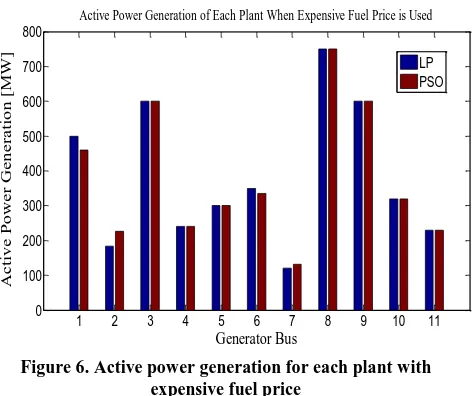
Figure 6. shows the generation of each plant for Linear Programming method compared with Particle Swarm Optimization when expensive fuel price is used.
0 5 10 15 20 25
0.95 0.96 0.97 0.98 0.99 1 Buses V o lt a g e M a g n it u d e [p .u .]
Voltage Magnitude of Each Bus When Cheap Fuel Price is Used
LP PSO
1 2 3 4 5 6 7 8 9 10 11 0 200 400 600 800
Generator Bus
A c ti v e P o w e r G e n e ra ti o n [M W] Active Power Generation of Each Plant When Cheap Fuel Price is Used
LP PSO
PSO Model: Inertia Weighted PSO
Dimensions : 10
No. of particles : 50
Error : 1e-010
Function : iraqopf
Inertia Weight : 0.4005
0 200 400 600 800 1000
105.75 105.76 105.77 105.78
P
ro
d
u
ct
io
n
Co
st
[$
/h
]
555719 = iraqopf( [ 10 inputs ] )
Iteration
0 5 10 15 20 25
0.95 0.96 0.97 0.98 0.99 1
Buses
V o lt a g e M a g n it u d e [p .u .]Voltage Magnitude of Each Bus When Expensive Fuel Price is Used
[image:4.595.48.288.349.744.2] [image:4.595.310.562.376.533.2] [image:4.595.54.287.574.740.2]Figure 6. Active power generation for each plant with expensive fuel price
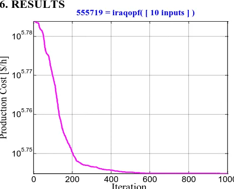
[image:5.595.54.291.314.495.2]Figure 7. shows the variation of production cost through optimization using Particle Swarm Optimization (PSO).
Figure 7. Production cost when expensive fuel price is used
Table 2 Results when cheap fuel price is used
LP PSO
Total Active Gen. 4191.061 [MW] 4190.741[MW] Total Reactive Gen. 47.24 [Mvar] 27.9 [Mvar] Total Active Load 4177 [MW] 4177 [MW] Total Reactive Load 1998 [Mvar] 1998 [Mvar] Total Active Loss 14.061 [MW] 13.741 [MW] Total Reactive Loss 123.83 [Mvar] 120.81 [Mvar] Production Cost
($/h)
564579.1 555719
Table 3 Results when expensive fuel price is used
LP PSO
Total Active Gen. 4193.914 [MW] 4194.318 [MW] Total Reactive Gen. 71.67 [Mvar] 60.7 [Mvar] Total Active Load 4177 [MW] 4177 [MW] Total Reactive Load 1998 [Mvar] 1998 [Mvar] Total Active Loss 16.914 [MW] 17.318 [MW] Total Reactive Loss 149.59 [Mvar] 153.07 [Mvar] Production Cost ($/h) 800448.87 787996
7. CONCLUSIONS
The Particle Swarm Optimization (PSO) algorithm is used for the first time on the Iraqi Extra High Voltage (EHV 400kV) Grid for optimal power flow to minimize the active power generation cost. paper has presented a PSO based.
The problem constraints are the coupled power flow equations and the system variable limits. .
It can be also note that the results of the production cost are significantly decreased when using Particle Swarm Optimization (PSO) with the results derived in the case of Linear Programming (LP) Method. From Table 2 there is about 1.57% decrease in the production costs when using cheap fuel type, whereas there is about 1.556% decrease in production costs when using expensive fuel type as given in Table 3.
8. REFERENCES
[1] B. R. Barkovich and D. Hawk, Charting a New Course in California, IEEE Spectrum, Vol. 33, No. 7, July 1996, pp. 26-31.
[2] M. G. Morgan and S. Talukdar, Nurturing R&D, IEEE Spectrum, Vol. 33, No.7, July 1996, pp. 32-33.
[3] H. Rudnick, Pioneering Electricity Reform in South America, IEEE Spectrum, Vol. 33, No. 8, August 1996, pp. 38-44.
[4] Acha, E., Ambriz-Pe´rez, H., Fuerte-Esquivel, C.R., Advanced Trans-former Control Modeling in An Optimal Power Flow Using Newton’s Method, IEEE Trans. Power Systems 15(1), pp. 290–298, 2000.
[5] Huneault, M., Galiana, F.D., A Survey of the Optimal Power Flow Literature, IEEE Trans. Power Systems 6(2), pp. 762–770, 1991.
[6] Monticelli, A., Liu,W.H.E., Adaptive Movement Penalty Method for the Newton Optimal Power Flow, IEEE Trans. Power Systems,Vol.7(1), pp. 334–342, 1992. [7] El-Hawary, M.E., Tsang, D.H., The Hydro-Thermal
Optimal Power Flow, A Practical Formulation and Solution Technique Using Newton’s Approach, IEEE Trans. Power Systems PWRS-1(3), pp. 157–167, 1986. [8] J. Carpienter, Contribution e l’étude do Dispatching
Economique, Bulletin Society Française Electricians, Vol. 3, August 1962.
[9] J. Wood and B. F. Wollenberg, Power Generation Operation and Control, New York, NY: John Wiley & Sons, Inc., pp. 39-517, 1996.
[10]H.W .Dommel and W. F. Tinney, Optimal Power Flow Solutions, IEEE Transactions on Power Apparatus and Systems, Vol. PAS-87, October 1968, pp. 1866-1876. [11]D. I. Sun, B. Ashley, B. Brewer, A. Hughes and W. F.
Tinney, Optimal Power Flow by Newton Approach, IEEE Transactions on Power Apparatus and Systems, Vol. PAS-103, October 1984, pp. 2864-2880.
[12]O. Alsac, J. Bright, M. Prais and B. Stott, "Further Developments in LP-Based Optimal Power Flow", IEEE Transactions on Power Systems, Vol. 5( 3), pp. 697-711, 1990.
[13]J. Kennedy and R. C. Eberhart, Particle swarm optimization, Proceedings of the 1995 IEEE International
1 2 3 4 5 6 7 8 9 10 11
0 100 200 300 400 500 600 700 800
Generator Bus
A
c
ti
v
e
P
o
w
e
r
G
e
n
e
ra
ti
o
n
[M
W
]
Active Power Generation of Each Plant When Expensive Fuel Price is Used
LP PSO
0 200 400 600 800 1000
105.9 105.91 105.92
Iteration
P
ro
d
u
ct
io
n
Co
st
[$
/h
]
787996 = iraqopf( [ 10 inputs ] )
PSO Model: Inertia Weighted PSO
Dimensions : 10
No. of particles : 50
Error : 1e-010
Function : iraqopf
Inertia Weight : 0.4005
Conference on Neural Networks, IEEE Service Center, Piscataway, NJ, 1995.
[14]S. Rao Singiresu: Engineering Optimization Theory and Practice, John Wiley & Sons, 2009.
[15]Jizhong Zho , "optimization of power system operation", Institute of Electrical and Electronics Engineers John Wiley & Sons, Inc., Hoboken, New Jersey, 2009. [16]Y. Shi and R. Eberhart: Parameter Selection in Particle