IMAGE DUPLICATION AND ROTATION DETECTION METHODS FOR STORAGE UTILIZATION

(1)

ISSN:1992-8645 www.jatit.org E-ISSN:1817-3195

AN INSIGHT INTO ADAPTIVE NOISE CANCELLATION

AND COMPARISON OF ALGORITHMS

1_{M. L. S. N. S. LAKSHMI,}2_{P. MICHAEL PREETAM RAJ,}3_{RAKESH TIRUPATHI,}

4_{P. GOPI KRISHNA,}5_{K.V.L. BHAVANI,}

1, 2, 3_{Assistant Professor, Department of ECE, KL University, Vijayawada, India}

4

Assistant Professor, Department of ECM, KL University, Vijayawada, India

5

Graduate Engineering Student, Electrical Engineering Dept., Santa Clara University, Santa Clara, USA

E-mail:[email protected],[email protected],[email protected]

,

4

gopikrishna.popuri@ kluniversity.in,[email protected]

ABSTRACT

The principle of adaptive noise cancellation is to acquire an estimation of the unwanted interfering signal and subtract it from the corrupted signal. Adaptive Noise Cancellation technique is an approach for powerful noise cancellation. In this paper the noise cancellation is performed using adaptive noise cancellers using an adaptive finite impulse response (FIR) filter are presented for the estimation of a transfer function of a noisy channel in a communication link. Optimizations of the Least Mean Square (LMS) versions and Normalized LMS (NLMS), Weiner algorithms are also used to adapt the filter coefficients of the estimated transfer functions in order to minimize the effect of background noise effectively & analyzed their performances with respect to their estimation of weights.

Keywords: Finite Impulse response filters (FIR), Infinite Impulse response filters (IIR), Least-mean square

algorithm (LMS), Normalized least mean square algorithm (NLMS), WIENER algorithm

1. INTRODUCTION

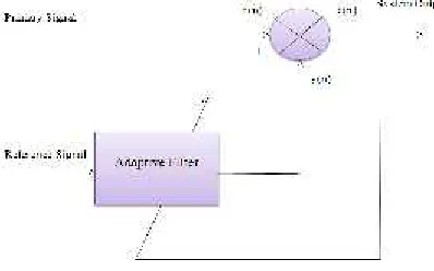
[image:1.612.92.291.577.701.2]

A Digital communication system consists of a transmitter, receiver and channel connected together. Typically the channel suffers from two major kinds of impairments: Inter symbol interference and Noise. Adaptive noise cancellation a specific type of interference cancellation uses cancellation of noise by subtracting noise from a received signal, an operation which is controlled in a manner which is adaptive for the purpose of improved signal to noise ratio (SNR). It is basically a dual-input, closed loop adaptive control system as shown in Figure 1.

Figure 1: Noise Cancellations

Here the adaptive filter is used to cancel unknown interference contained in a primary signal, with the cancellation being optimized in smarter sense. The basic signal serves as the required response of the filter. The reference signal is the input to this filter. This paper studies and compares the performance analysis of three adaptive algorithms in noise cancelling. Simulations done based on different types of signals mixed with various types of noise & their response after application of three adaptive filters and are presented.

2. ADAPTIVE NOISE CANCELLER

(2)

[image:2.612.95.312.72.232.2]

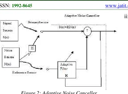
Figure 2: Adaptive Noise Canceller

As shown in above figure 2 the primary sensor not only records the signal from the required signal source but also picks up a delayed and/ or filtered noise originating from the noise source.

Recorded signal at primary sensor = S (n) +HN (n)

Let V (n)= HN (n) represents the noise signal at primary sensor and assume the desired signal and noise signal are uncorrelated with each other such that,

E [S (n) V (n-m)] = 0 for all m Noise signal N (n) originated at the reference sensor is uncorrelated with signal S (n) i.e.

E [s (n) N (n-m)] = 0 for all m However N (n) is correlated with delayed and filtered noise V (n) or HN (n) at the primary sensor output in an unknown way such that,

E [V (n) N (n-m)] = p (m) for all m

Where p(m) is unknown-correlation for lag m.

S*(n) = S (n) + HN (n)–H*N (n) = S (n) + (H-H*)

N (n) = e (n) (1)

From equation, the essential noise component is (H-H*) N (n). This term can be minimized if H = H*, which in turn leads to maximization of system output signal-to- noise (SNR) ratio.

The adaptive noise cancellation system and its effectiveness depend on the following important factors:

i. The signal and noise at the output of the primary sensor are uncorrelated.

ii. The noise signal recorded at the reference sensor is highly correlated with the noise component in the primary sensor output.

iii. The desired signal component in the primary sensor output is undetectable a reference sensor.

After examining the rudimentary operation of noise cancellation device different types of algorithms which are required to implement the noise cancellation problem are presented in [1]. This type of noise cancellation which makes use of

DSP’s are known as adaptive filtering problem[1]. The different kinds of adaptive filter algorithms are LMS, NLMS and WIENER. These algorithms are discussed in the subsequent chapters.

3. ADAPTIVE FILTERS

By this we can define the term “adaptive

filter” as the filter whose characteristics can be

modified or altered to achieve an objective by automatic adaptation or modification of the filter parameters [2].

Adaptive filters are often realized as a set of program instructions running on an arithmetical processing device such as a microprocessor or a DSP chip or a set of logical operations implemented in a field programmable gate array (FPGA) or in a semi-custom or custom VLSI integrated circuit, the fundamental operation of an adaptive filter can be characterized independently of the specific physical realization that it takes [3].

The adaptive noise cancelling concept, an alternative method which estimating signals corrupted by interference or additive noise, where this method uses a primary input which contains the corrupted signal and a reference input having noise correlated in an unknown way with the primary noise is presented in [4].

The problem of noise cancellation and arrhythmia detection in ECG, using adaptive filtering techniques which are computationally simplified is presented in [5].

4. CLASSIFICATION OF ADAPTIVE

FILTERS

The two most fundamental types of adaptive filters are:

(3)

5. FINITE IMPULSE RESPONSE FILTERS

(FIR)

FIR filter get their name from naturally enough- the way they respond to their impulse. It is an input of value 1 lasting just to be sampled only once and only once of the response of the filter is finite then we say that filter is FIR filter. From practical point of view, finite response means that, when a unit impulse is given to a filter, the output response should return to zero after some time2. We can write output signal y (n) as,











L 1

0 i

i

(n)x(n

i)

w

y(n)

(2)

y (n) = w0 (n) x (n-0) + w1 (n) x (n-1) + w2(n) x (n-2)…... wL-1(n) x (n-L+1) (3)

y (n) = WT(n) X (n) (4)

Where,

W (n) = the impulse response values of filter at time n.

X (n) = [x (n), x (n-1)… x (n-L+1]Tdenotes input signal vector and T denotes the vector transpose [2].

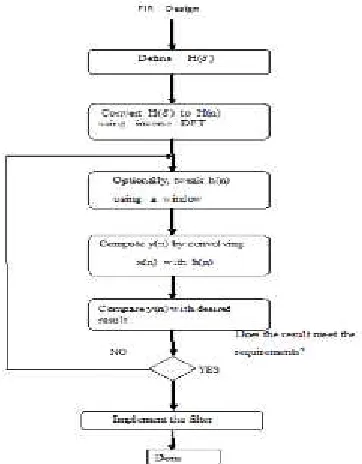
Where, h (n) = is the transfer function

H (n) = transfer function converted into frequency form

[image:3.612.101.282.477.709.2]

y (n) = filter output

Figure 3: Algorithm for FIR filter

6. ALGORITHMS

The three famous algorithms are: 1. Weiner algorithm

2. LMS algorithm 3. NLMS algorithm

6.1 The Wiener Solution

For the FIR filter structure, the coefficient values in W (n) that minimize JMSE (n) are well-defined if the statistics of the input and desired response signals are known. The formulation of this problem for continuous-time signals and the resulting solution was first derived by Wiener. Hence, this optimum coefficient vector WMSE(n ) is often called the Wiener solution to the adaptive filtering problem [6].

To determine WMSE(n), we note that the function JMSE(n) in is quadratic in the parameters {wi(n)} , and the function is also differentiable. Thus, WMSE(n) can be found from the solution to the system of equations [6]

0,

(n)

w

J

i MSE(n)





1 L

i

0 





(5)



















)

(

)

(

)

(

)

(

)

(

n

w

n

e

n

e

E

n

w

n

J

i i MSE

.

)

(

)

(

)

(

{

)}

(

)

(

{

1

0



















  L j j

n

w

j

n

x

i

n

x

E

i

n

x

n

d

E

.

The matrix Rxx(n) and vector Pdx(n) are defined as

)}

(

)

(

{

)

(

n

E

x

n

X

n

R

xx



T (6)

)},

(

)

(

{

)

(

n

E

d

n

X

n

P

dx



₍₇₎

We can combine these two terms to obtain the system of equations in vector form as

0 (n)

P

(n)

(n)W

R

_XX _MSE



_dX



Where



is the zero vector. As long as the Rxx(n) matrix is invertible, the optimum Wiener solution vector for this problem is

(n)

(n)P

R

(n)

(4)

A detailed discussion on the Wiener filter’s

quantitative performance behavior in the context of reduction of noise is given in [7].

6.2 Least Mean Square Algorithm:

LMS (Least mean square), an adaptive algorithm, uses a gradient-based method providing steepest decent. It uses the estimates of the gradient vector from the available data.

LMS incorporates an iterative procedure that makes successive corrections to the weight vector in the direction of the negative of the gradient vector which eventually leads to the mean square error which is of minimum value. LMS algorithm is relatively simpler compared to other algorithms; it does not require correlation function calculation nor does it require matrix inversions [3].

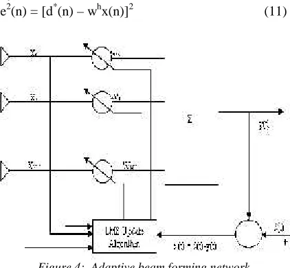
Consider a Uniform Linear Array (ULA) with N isotropic elements forming the adaptive beamforming system’sintegral part as shown in the below figure 4.

The antenna array’soutput is given by,









Nu

i

t

a

n

t

u

a

t

s

t

x

1

0

)

(

)

(

)

(

)

(

)

(

)

(



(9)

a (



₀ ) and a (



₁ ) represents the steering vectors

for the desired signal and interfering respective signals. Therefore the desired signal is to be construct the from the received signal amid the interfering signal and additional noise n(t) [8]. As shown in figure 4 above the outputs of the individual sensors are linearly combined after being scaled using corresponding weights such that the antenna array pattern is optimized to have maximum possible gain in the direction of the desired signal and nulls in the direction of the interferers.

From the steepest descent’s method, the weight vector equation is given by

)})]

(

{

(

[

2

1 )

(

)

1 (

n

w

n

E

e

2

n

w











(10)

Where µ, controlling is the step-size parameter, is the convergence characteristics of the LMS algorithm

e2(n) is error in mean square about the beam former output y(n) and the reference signal which is given by,

[image:4.612.313.524.184.379.2]

e2(n) = [d*(n)–whx(n)]2 (11)

Figure 4: Adaptive beam forming network

The above weight update equation’sgradient vector can be computed as

2Rw(n)

2r

(n)})

(E{e

2

w









(12)

In the method of steepest descent the biggest problem is the computation involved in finding the values r and R matrices in real time. On the other hand, the LMS algorithm simplifies this by using the instantaneous values of covariance matrices r and R instead of their actual values i.e.

R (n) = x(n)xh(n) r (n) = d*(n) x (n)

Therefore the update weights of can be given by the equation,

w(n+1) = w (n) + µx (n) e*(n) (18)

(5)

The weight vector’s successive corrections eventually lead to the minimum value of the mean squared error [8].

Therefore the summarization of LMS algorithm can be in following equations;

Output, y (n) = whx(n) (13)

Error, e (n) = d*(n)–y (n) (14)

Weight, w (n+1) = w (n) + µx (n) e*(n) (15) An adaptive noise cancellation method having two stages, for enhancing an ideal signal submerged in noise, where the overall method uses two adaptive filters with reference and primary signals [9].

An insight into an algorithm combining multi-channel differencing and thus obtaining reference noise and KNLMS which adaptively cancel the unknown noise is presented in [10].

7. SIMULATION RESULTS & DISCUSSION

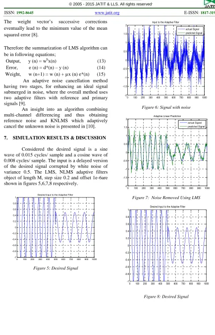
Considered the desired signal is a sine wave of 0.015 cycles/ sample and a cosine wave of 0.008 cycles/ sample. The input is a delayed version of the desired signal corrupted by white noise of variance 0.5. The LMS, NLMS adaptive filters object of length M, step size 0.2 and offset 1e-6are shown in figures 5,6,7,8 respectively.

0 100 200 300 400 500 600 700 800 900 1000 -1

-0.8 -0.6 -0.4 -0.2 0 0.2 0.4 0.6 0.8

1 Desired Input to the Adaptive Filter

Figure 5: Desired Signal

0 100 200 300 400 500 600 700 800 900 1000 -2

-1.5 -1 -0.5 0 0.5 1 1.5

2 Input to the Adaptive Filter

actual Signal predicted Signal

Figure 6: Signal with noise

0 100 200 300 400 500 600 700 800 900 1000 -2

-1.5 -1 -0.5 0 0.5 1 1.5

2 Adaptive Linear Prediction

Figure 7: Noise Removed Using LMS

0 100 200 300 400 500 600 700 800 900 1000 -1

-0.8 -0.6 -0.4 -0.2 0 0.2 0.4 0.6 0.8

[image:5.612.82.516.56.731.2]

1 Desired Input to the Adaptive Filter

(6)

0 100 200 300 400 500 600 700 800 900 1000 -2

-1.5 -1 -0.5 0 0.5 1 1.5

2 Input to the Adaptive Filter

Figure 9: Signal with noise

0 100 200 300 400 500 600 700 800 900 1000 -2

-1.5 -1 -0.5 0 0.5 1 1.5

2 Adaptive Linear Prediction

[image:6.612.90.521.58.654.2]

Figure 10: Noise removed using NLMS

0 200 400 600 800 1000 1200 1400 1600 1800 2000 10-7

10-6 10-5 10-4 10-3 10-2 10-1

100 Error curve

Samples

E

rro

r v

al

ue

Figure 11: Estimation Error using LMS

0 200 400 600 800 1000 1200 1400 1600 1800 2000 -2

-1.5 -1 -0.5 0 0.5 1

1.5 System output

Samples

T

ru

e

a

n

d

e

s

ti

m

a

te

d

o

u

tp

u

t

Figure 12: System Output’s Signal Spectrum-LMS

0 1 2 3 4 5 6

0.05 0.1 0.15 0.2 0.25 0.3

Comparison of the actual weights and the estimated weights

[image:6.612.325.517.328.506.2]

Actual weights Estimated weights

Figure 13: Comparison of LMS Weight

[image:6.612.103.287.471.657.2]

(7)

0 200 400 600 800 1000 1200 1400 1600 1800 2000 10-5

10-4 10-3 10-2 10-1

100 Error curve

Samples

E

rr

or

v

al

[image:7.612.94.311.59.685.2]

ue

Figure 14: Estimation Error using NLMS

0 200 400 600 800 1000 1200 1400 1600 1800 2000 -2

-1.5 -1 -0.5 0 0.5 1

1.5 System output

Samples

Tr

ue

a

nd

e

st

im

at

ed

o

ut

pu

[image:7.612.100.291.322.461.2]

t

Figure 15: System Output’s spectrum-NLMS

900 910 920 930 940 950 960 970 980 990 1000 -1.5

-1 -0.5 0 0.5 1 1.5

Time index (n)

A

m

pl

itu

de

Wiener filter denoised sinusoid LMS denoised sinusoid NLMS denoised sinusoid

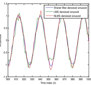
Figure 16: Comparison of Wiener-LMS& NLMS Algorithms

8. CONCLUSION

The adaptive filtering techniques are using in almost every electronic equipment. So it has become imperative to develop an algorithm for the adaptive filter.

We have explored different ways of finding a suitable adaptive filter algorithm which improves the adaptive filter performance. All the parameters regarding the adaptive filter algorithms are calculated. First the LMS algorithm discussed was most widely used, as it is computationally easy and numerically robust. But this algorithm has a disadvantage that the rate of convergence of this algorithm is very slow.

NLMS algorithm is a better choice as it has a better rate of convergence compared to the LMS algorithm. From the Figure 16 we can conclude that Wiener algorithm is a better algorithm compared to NLMS algorithm by considering the estimation weights & errors. New knowledge this work has created is that Weiner filter is the best noise reduction filter which can be used in the fields of signal processing.

[image:7.612.102.295.494.675.2]

(8)

REFERENCES:

[1] S.C. Douglas and R. Losada,"Adaptive Filters in MATLAB: From Novice to Expert," PROC. 2ND. Signal Processing Education Workshop, Callaway Gardens, GA,PAPER4.9,

OCTOBER2002.

[2] Nicholson, B. W., Upton, David M., Cotterill, Steve, Marchese, Jim, Upadhyay, Triveni, Velde, Wallace E. Vander, "Computer Simulation of Digital Beam Forming Adaptive Antennae for GPS Interference Mitigation," Proceedings of the 1998 National Technical Meeting of The Institute of Navigation, Long Beach, CA, January 1998, pp. 355-360.

[3] Islam, s.z, jidin.r, Ali M.“Performance study of adaptive filtering algorithms for noise cancellation of ECG signal”, IEEE International conference on communication & signal processing 2009, P.1-5.

[4] Widrow , J. R. Glover Jr, J. M. McCool , J. Kaunitz , C. S. Williams , R. H. Hearn , J. R. Zeidler , E. Dong Jrand R. C. Goodlin "Adaptive noise cancelling: Principles and applications ", Proc. IEEE, vol. 63, pp.1692 -1717 1975.

[5] Md. Zia Ur Rahman, Rafi Ahamed Shaik and D V Rama Koti Reddy "Noise Cancellation in ECG Signals using Computationally Simplified Adaptive Filtering Techniques: Application to Biotelemetry" in Signal Processing: An International Journal (SPlJ)

Volume 3, Issue 5, pp. 120.

[6] V. R VIJAY KUMAR, P. KANAGASABAPATHYP.

T. VANATHI,“MODIFIEDADAPTIVEFILTERING

ALGORITHM FOR NOISE CANCELLATION IN

SPEECH SIGNALS”, ELECTRONICS AND

ELECTRICAL ENGINEERING, KANUS:

TECHNOLOGIJA, 2007. NO. 2(74). P.17-20. [7] Chen , J. Benesty , Y. Huang and S. Doclo

"New insights into the noise reduction Wiener filter", IEEE Trans. Audio, Speech, Lang.

Process., vol. 14, no. 4, pp.1218 -1234 2006.

[8] Ying He, Hong He, "The Applications and Simulation of Adaptive Filter in Noise Canceling", Embedded Programming, 2008

International Conference on Computer Science and Software Engineering (CSSE 2008).Vol.4.pp.1-4.

[9] Xueli Wu, Zizhong Tan ; Jianhua Zhang ; Wei Li, “Dual adaptive noise cancellation method

based on Least Mean M-estimate of noise”,

Intelligent Control and Automation (WCICA), 2014 11th World Congress on June 29, 2014-July 4, 2014, pp.5741–5746.

[10] Jianguo Huang, Wei Gao, Richard. C