Study of University Dropout Reason Based on Survival Model

(1)

ISSN Online: 2161-7198 ISSN Print: 2161-718X

DOI: 10.4236/ojs.2016.65075 October 24, 2016

Study of University Dropout Reason Based on

Survival Model

Juan C. Juajibioy

Fundación Universidad Autónoma de Colombia, Bogotá, Colombia

Abstract

In this paper, we introduce the survival modelling methodology in order to identify some factors which may be influencing the university dropout. By using the data base provided by the Fundación Universidad Autónoma de Colombia and the semi parametric proportional hazard Cox model, we have been able to identify these risk factors.

Keywords

Dropout, Survival Models

1. Introduction

According to SPADIES1_{in Colombian Institutions Higher Education, around 20% of} students beginning an undergraduate program drop out at first year. That is a global phenomenon: usually the group of graduates is smaller respect to the number of begin-ners. That is due to variables of academic, social or economic type and several studies have been realized about it. From this global phenomenon arose two big questions:

• _{What are the factors influencing the student drop out?} • _{How long take a student to drop out university?}

The most literature about the first question is divided in two branches: Tinto’s stu-dent integration model and Bean and Metzner’s stustu-dent attrition model (1985). The first one refers to the student’s integration process and the second one refers to the student’s individual variables, see [1] [2] and references therein for a detailed descrip-tion.

Respect to the second question, the survival models have been amply developed, and typically focused on time to event data.

1_{Sistema para Prevención de la Deserción de la Educación Superior}

How to cite this paper: Juajibioy, J.C. (2016) Study of University Dropout Reason Based on Survival Model. Open Journal of Statis-tics, 6, 908-916.

http://dx.doi.org/10.4236/ojs.2016.65075

Received: July 28, 2016 Accepted: October 21, 2016 Published: October 24, 2016

(2)

2. Discrete Duration Analysis

Following [3] [4] we introduce the necessary background. Let T be the discrete variable representing the duration of studies (by semester from 1 until 12). The survival func-tion is defined as

( )

(

)

.

S t =P T>t

(1)

Since p t

( )

k =P T

(

=tk

)

we have

( )

(

)

( )

.

k

t t

S t P T t p t

>

= > =

∑

(2)

The Hazard function is defined as

( )

(

1

)

_{( )}

( )

1

| k .

k k k

k

p t h t P T t T t

S t

−

= = > = ₍₃₎

Notice that P T

(

≥tk

)

=S t

( )

k−1 , since p t

( )

k =S t

( ) ( )

k−1 −S tk , by using (3) we have

( )

1

( )

1 , k k k S t h t

S t ₋ = − (4)

so, the survival function can be written as

( )

(

1

( )

)

k

t t

S t h t

≤

=

∏

− (5)

2.1. The Nonparametric Kaplan-Meyer Estimator

Let ti the failure time, di the number of events that occur at time ti and ni the

number of individuals at risk of experiencing the event immediately prior to tj, then the product limit estimator of survival function is

( )

ˆ _.

j

j j

t t j

n d S t n <  −  = _ _  

∏

(6)

An interesting representation is given in [3] by using the following table

j

t nj mj S tˆ

( )

j

0 0

t = n0 0 1



k

t nk mk S tˆ( )k where n0 is the initial population.

2.2. The Nonparametric Cox’s Proportional Hazard Model

The Cox’s proportional hazard model really gives a semi parametric method to the es-timate the hazard function at time t given a baseline hazard that’s modified by a set of covariates:

(

|

)

0

( )

exp

(

1 1 n n

)

0

( )

exp

(

)

(3)

where h t0

( )

is the non-parametric baseline hazard function X =

(

X1,,Xn

)

is a set

of explanatory variables

3. Data and Descriptive Analysis

In this section we defined the principal explanatory variables and consider some de-scriptive aspects of these variables. We take a set that belong a cohort of students that began the studies in the first semester of 2010 in the University Fundación Universidad Autónoma de Colombia. In order to differentiate the group of students, we consider the following groups

• _{Group 1, Graduated Students: Student which finished successful their studies before}

12 semesters.

• _{Group 2, Active students: In the dataset in second semester of 2015.}

• Group 3, Inactive Students: Students who did not register for more than three con-secutive semesters in the dataset.

In our analysis the following covariates were collected, grouped by individuals and academics. We consider the following individual variables

Variables Individuals Gender Age Social status Location

0 for female and 1 for male.

Age of the student when beginning his studies. In Colombia there are six class of social status. Location of student’s home.

academics

P1 P2 P3 Picfes

Grade point average at first semester. Grade point average at second semester. Grade point average at second semester. Score in icfes tests.

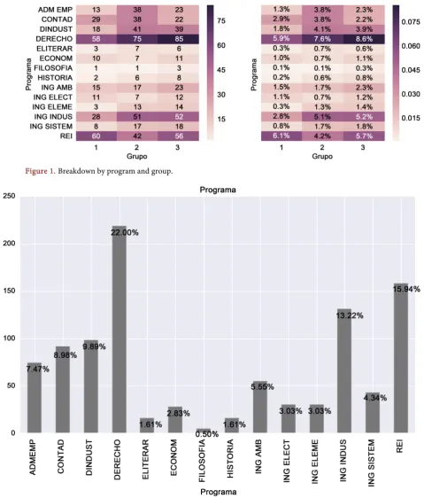
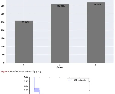
A breakdown by program and group is given in Figure 1. And in Figure 2, we show the percent of students by program.

In Figure 2 we present the percent of students that began their studies at first seme-ster of 2010.

(4)

4. Duration Analysis

[image:4.595.77.557.127.690.2]

In this section we looking for the relationship between the student’s decision to com-plete or abandon, opposite to the decision of prolong their permanence at university.

Figure 1. Breakdown by program and group.

(5)

[image:5.595.101.558.89.460.2] [image:5.595.195.466.387.573.2]

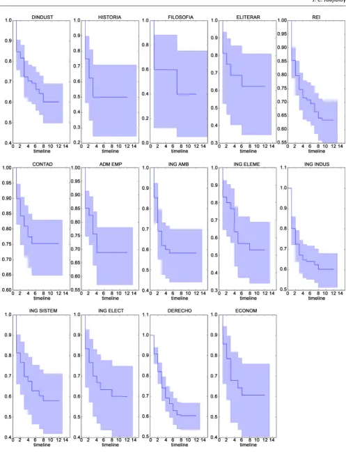
Figure 3. Distribution of students by group.

Figure 4. Kaplan Meier estimate for Survival function.

Initially we used the nonparametric Kaplan-Meier estimator 2.6, the results are given in Table 1 (See Appendix)

In Figure 4 it can see that the bigger drooping out rate occurs during the four initial semesters. In Figure 5 it is possible see the dynamics of survival in all programs that university offers

(6)

[image:6.595.55.553.49.698.2]

(7)

[image:7.595.149.555.62.338.2]

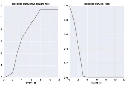
Figure 6. Baseline cumulative hazard and survival rate.

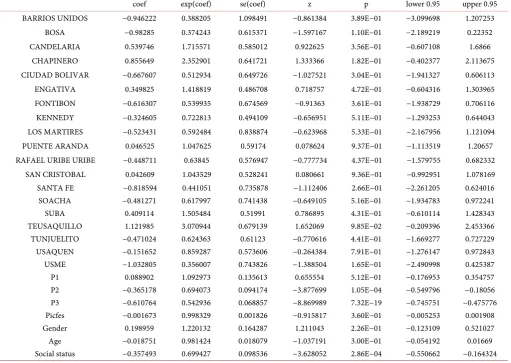
results can see in Table 2 (See Appendix)

The baseline cumulative hazard H t

( )

=

∑

t_j<th t0

( )

it can see in Figure 6, notice in the left side the rapidly increasing rate, meaning that the hazard increase during the four first semesters.

5. Conclusion

In this work, we use the nonparametric survival model in order to estimate the risk factors for the university drop out, factors such that grade point average at first seme-ster, gender and location are most significant in our study, remember that a positive es-timate in the coefficient indicates an increased hazard meaning shorter expected sur-vival time. By gender, the male population has more hazards to sursur-vival than female population. Finally after accounting for age, sex, grade point average and location there are no statistically significant associations between Icfes score and Social status and all- cause drop out.

Acknowledgements

This research was supported by SUI: Sistema Universitario de Investigación, Fundación Universidad Autónoma de Colombia.

Conflict of Interest

(8)

References

[1] Montoya Diaz, M. (1999) Extended Stay at University: An Application of Multinomial Logit and Duration Models. Applied Economics, 31, 1411-1422.

http://dx.doi.org/10.1080/000368499323292

[2] Giovagnoli, P. (2005) Determinants in University Desertion and Graduation: An Applica-tion Using DuraApplica-tion Models. Ecónomica LI, No. 1, 60-90.

[3] Kleinbaum, D. and Klein, M. (2005) Survival Analysis: A Self-Learning Text. Springer. [4] Pintilie, M. (2006) Competing Risks: A Practical Perspective. Wiley.

(9)

[image:9.595.220.377.110.311.2]

Appendix

Table 1. KM Estima for survival function.

j

t S tˆ

( )

_j

0 1.000000

1 0.855701

2 0.788093

3 0.722503

4 0.686176

5 0.667850

6 0.653172

7 0.637957

8 0.622397

9 0.621255

10 0.621255

11 0.621255

12 0.621255

Table 2. Hazard ratios.

coef exp(coef) se(coef) z p lower 0.95 upper 0.95

BARRIOS UNIDOS −0.946222 0.388205 1.098491 −0.861384 3.89E−01 −3.099698 1.207253

BOSA −0.98285 0.374243 0.615371 −1.597167 1.10E−01 −2.189219 0.22352

CANDELARIA 0.539746 1.715571 0.585012 0.922625 3.56E−01 −0.607108 1.6866

CHAPINERO 0.855649 2.352901 0.641721 1.333366 1.82E−01 −0.402377 2.113675

CIUDAD BOLIVAR −0.667607 0.512934 0.649726 −1.027521 3.04E−01 −1.941327 0.606113

ENGATIVA 0.349825 1.418819 0.486708 0.718757 4.72E−01 −0.604316 1.303965

FONTIBON −0.616307 0.539935 0.674569 −0.91363 3.61E−01 −1.938729 0.706116

KENNEDY −0.324605 0.722813 0.494109 −0.656951 5.11E−01 −1.293253 0.644043

LOS MARTIRES −0.523431 0.592484 0.838874 −0.623968 5.33E−01 −2.167956 1.121094

PUENTE ARANDA 0.046525 1.047625 0.59174 0.078624 9.37E−01 −1.113519 1.20657

RAFAEL URIBE URIBE −0.448711 0.63845 0.576947 −0.777734 4.37E−01 −1.579755 0.682332

SAN CRISTOBAL 0.042609 1.043529 0.528241 0.080661 9.36E−01 −0.992951 1.078169

SANTA FE −0.818594 0.441051 0.735878 −1.112406 2.66E−01 −2.261205 0.624016

SOACHA −0.481271 0.617997 0.741438 −0.649105 5.16E−01 −1.934783 0.972241

SUBA 0.409114 1.505484 0.51991 0.786895 4.31E−01 −0.610114 1.428343

TEUSAQUILLO 1.121985 3.070944 0.679139 1.652069 9.85E−02 −0.209396 2.453366

TUNJUELITO −0.471024 0.624363 0.61123 −0.770616 4.41E−01 −1.669277 0.727229

USAQUEN −0.151652 0.859287 0.573606 −0.264384 7.91E−01 −1.276147 0.972843

USME −1.032805 0.356007 0.743826 −1.388504 1.65E−01 −2.490998 0.425387

P1 0.088902 1.092973 0.135613 0.655554 5.12E−01 −0.176953 0.354757

P2 −0.365178 0.694073 0.094174 −3.877699 1.05E−04 −0.549796 −0.18056

P3 −0.610764 0.542936 0.068857 −8.869989 7.32E−19 −0.745751 −0.475776

Picfes −0.001673 0.998329 0.001826 −0.915817 3.60E−01 −0.005253 0.001908

Gender 0.198959 1.220132 0.164287 1.211043 2.26E−01 −0.123109 0.521027

Age −0.018751 0.981424 0.018079 −1.037191 3.00E−01 −0.054192 0.01669

[image:9.595.44.556.346.709.2]