http://dx.doi.org/10.4236/am.2014.58111
Automatic Clustering Using
Teaching Learning Based
Optimization
M. Ramakrishna Murty
1, Anima Naik
2, J. V. R. Murthy
3, P. V. G. D. Prasad Reddy
4,
Suresh C. Satapathy
5, K. Parvathi
61GMR Institute of Technolgy, Rajam, India
2Majhighariani Institute of Technology & Science, Rayaged, India 3Jawaharlal Nehru Technological University, Kakinada, India 4Andhra University, Visakhapatnam, India
5Anil Neerukonda Institute of Technology and Sciences, Visakhapatnam, India 6Centurion University of Technology and Management, Paralakhemundi, India
Email: [email protected], [email protected], [email protected], [email protected], [email protected], [email protected]
Received 8 March 2014; revised 8 April 2014; accepted 15 April 2014
Copyright © 2014 by authors and Scientific Research Publishing Inc.
This work is licensed under the Creative Commons Attribution International License (CC BY). http://creativecommons.org/licenses/by/4.0/
Abstract
Finding the optimal number of clusters has remained to be a challenging problem in data mining research community. Several approaches have been suggested which include evolutionary com- putation techniques like genetic algorithm, particle swarm optimization, differential evolution etc. for addressing this issue. Many variants of the hybridization of these approaches also have been tried by researchers. However, the number of optimal clusters and the computational efficiency has still remained open for further research. In this paper, a new optimization technique known as “Teaching-Learning-Based Optimization” (TLBO) is implemented for automatic clustering of large unlabeled data sets. In contrast to most of the existing clustering techniques, the proposed algo- rithm requires no prior knowledge of the data to be classified rather it determines the optimal number of partitions of the data “on the run”. The new AUTO-TLBO algorithms are evaluated on
benchmark datasets (collected from UCI machine repository) and performance comparisons are
made with some well-known clustering algorithms. Results show that AUTO-TLBO clustering techniques have much potential in terms of comparative results and time of computations.
Keywords
1. Introduction
Clustering technique enables one to partition unlabeled data set into groups of similar objects known as clusters. However, each cluster is clearly different from other clusters. Evolutionary computation techniques are widely used by researchers to evolve clusters in the complex data sets. However, there is no adequate research progress to determine the optimal number of clusters [1]. Clustering techniques based on evolutionary computations, mainly take the number of classes K as input instead of determining the same during the execution process. In most of the cases, determining the appropriate number of clusters in real time situation is difficult.
Clustering validity index is popularly used, in traditional methods, to determine the optimal number of clus- ters. An efficient clustering validity index provides global minima/maxima at the exact number of classes in the data set. However, this method is very expensive since it requires formation of clustering for a variety of possi- ble cluster number. In order to overcome the above-said issue, this paper proposes a clustering algorithm, where a number of trial solutions are provided with different cluster numbers along with cluster center coordinates for the same data set. Correction of each possible grouping is quantitatively evaluated with a global validity index, the CS measure [2]. Then, through the evolution mechanism, eventually, the best solutions start dominating the population, whereas the bad ones are eliminated. Ultimately, the evolution of solutions comes to a halt (i.e., converges) when the fittest solution represents a near-optimal partitioning of the data set with respect to the em- ployed validity index. In this way, the optimal number of classes along with the accurate cluster center coordi- nates can be located in one run of the evolutionary optimization algorithm. But one major issue with this method is that its performance depends heavily on the choice of a suitable clustering validity index.
In this paper, a new optimization technique TLBO is implemented for auto clustering and the performance of this is compared with other techniques like classical DE [3] improved differential evolution (ACDE) [4]. One standard hierarchical agglomerative clustering based on the linkage metric of average link [5], the genetic clus- tering with an unknown number of clusters K (GCUK) [6], the dynamic clustering PSO (DCPSO) [7]. The fol- lowing performance metrics have been used in the comparative analysis: 1) the accuracy of final clustering re- sults; 2) the speed of convergence; and 3) the robustness (i.e., ability to produce nearly same results over re- peated runs). Some real life data sets have been taken for testing. The rest of this paper is organized as follows. Section 2 describes the PSO, DE and TLBO. Section 3 outlines the representation of Automatic clustering algo- rithm. Section 4 describes experimental results on some data sets. Conclusions are provided in Section 5.
2. Basics of PSO, DE and TLBO
There have been many variants of PSO and DE available. However, in this section we emphasize only the basic techniques to give reader a feel of these techniques.
2.1. Particle Swarm Optimization
PSO can be considered as a swarm-based learning scheme [8]. In PSO learning process, each single solution is a bird referred to as a particle. The individual particles fly gradually towards the positions of their own and their neighbors’ best previous experiences in a huge searching space. It shows that the PSO gives more opportunity to fly into desired areas to get better solutions. Therefore, PSO can discover reasonable solutions much faster [9]. PSO define a proper fitness function that evaluates the quality of every particle’s position. The position, called the global best (gbest), is the one which has the highest value among the entire swarm. The location, called it as personal best (pbest), is the one which has each particle’s best experience. Based on every particle’s momentum and the influence of both personal best (pbest) and global best (gbest) solutions, every particle adjusts its veloc- ity vector at each iteration. The PSO learning formula is described as follows.
(
)
( )
(
( )
( )
)
(
( )
( )
)
, 1 , 1 rand pbest, , 2 rand gbest ,
i m i m i m i m m i m
V t+ = ⋅τ V t + ∗c ∗ t −X t + ∗c ∗ t −X t (1)
(
)
( )
(
)
, 1 , , 1
i m i m i m
X t+ =X t +V t+ (2)
2.2. Classical DE and Its Modification
The classical DE [10] is a population-based global optimization algorithm that uses a floating-point (real-coded) representation. The ith individual vector (chromosome) of the population at time-step (generation) t has d com- ponents (dimensions), i.e.
( )
,1( )
, ,2( )
, , ,( )
i t = Xi t Xi t Xi d t X (3)
For each individual vector Xk
( )
t that belongs to the current population, DE randomly samples three other individuals, i.e., Xi( )
t , Xj( )
t and Xm( )
t , from the same generation (for distinct k, i, j, and m). It then cal- culates the (component wise) difference of Xi( )
t and Xj( )
t , scales it by a scalar F (usually ∈ [0, 1]), andcreates a trial offspring Ui
(
t+1)
by adding the result to Xm( )
t . Thus, for the nth component of each vector.(
)
( )
(
( )
( )
)
( )
( )
, , ,
,
,
, if rand 0,1 1
, otherwise
m n i n j n n r
k n
k n
X t F X t X t C
U t
X t
+ − <
+ =
(4)
[ ]
0,1 rC ∈ is a scalar parameter of the algorithm, called the crossover rate. If the new offspring yields a better value of the objective function, it replaces its parent in the next generation; otherwise the parent is retained in the population, i.e.,
(
1)
(
( )
1 , if)
(
(
(
(
1)
)
)
)
(
(
( )
( )
)
)
, if 1
i i i
i
i i i
t f t f t
t
t f t f t
+ + >
+ =
+ ≤
U U X
X
X U X (5)
where f() is the objective function to be maximized.
To improve the convergence properties of DE, it has been tuned its parameters in two different ways here [11]. In the original DE, the difference vector
(
Xi( )
t −Xj( )
t)
is scaled by a constant factor F. The usual choice for this control parameter is a number between 0.4 and 1. For modified DE, this scale factor in a random manner in the range (0.5, 1) by using the relation( )
(
)
0.5 1 rand 0,1
F= × + (6)
where rand (0, 1) is a uniformly distributed random number within the range [0, 1].
In random scale factor (DERANDSF) can meet or beat the classical DE. Here the time variation of Cr may be expressed in the form of the following equation:
(
max min)
(
)
Cr= Cr −Cr × MAXIT−iter MAXIT (7)
where Crmax and Crmin are the maximum and minimum values of crossover rate Cr, respectively; iter is the current iteration number; and MAXIT is the maximum number of allowable iterations.
2.3. Teaching Learning Based Optimization
This optimization method is based on the effect of the influence of a teacher on the output of learners in a class [12]. Like other nature-inspired algorithms, TLBO is also a population based method that uses a population of solutions to proceed to the global solution. TLBO has been already applied to clustering [13]. For TLBO, the population is considered as a group of learners. In optimization algorithms, the population consists of different design variables [14]. In TLBO, different design variables will be analogous to different subjects offered to learn- ers and the learners’ result is analogous to the “fitness”, as in other population-based optimization techniques. The teacher is considered as the best solution obtained so far.
The process of TLBO is divided into two parts. The first part consists of the “Teacher Phase” and the second part consists of the “Learner Phase”. The “Teacher Phase” means learning from the teacher and the “Learner Phase” means learning through the interaction between learners.
2.3.1. Teacher Phase
As teacher is considered most knowledgeable person in the society, the best learner is mimicked as a teacher. The teacher tries to disseminate knowledge among learners, which will in turn increase the knowledge level of the whole class and help learners to get good marks or grades. So a teacher increases the mean of the class according to his or her capability i.e. the teacher T1 will try to move mean M1 towards their own level according to his or her capability, thereby increasing the learners’ level to a new mean M2. Teacher T1 will put maximum effort into teaching his or her students, but students will gain knowledge according to the quality of teaching delivered by a teacher and the quality of students present in the class. The quality of the students is judged from the mean value of the population. Teacher T1 puts effort in so as to increase the quality of the students from M1 to M2, at which stage the students require a new teacher, of superior quality than themselves, i.e. in this case the new teacher is T2. Let Mi be the mean and Ti be the teacher at any iteration i. Ti will try to move mean Mi towards its own level, so now the new mean will be Ti designated as Mnew. The solution is updated according to the difference between the existing and the new mean given by
(
new)
Difference_meani=r Mi −T MF i (8)
where TF is a teaching factor that decides the value of mean to be changed, and ri is a random number in the range [0, 1]. The value of TF can be either 1 or 2, which is again a heuristic step and decided randomly with equal probability as
( ) (
)
round 1 rand 0,1 2 1 . F
T = + × − (9)
This difference modifies the existing solution according to the following expression
new ,i old,i Difference_meani
X =X + (10)
2.3.2. Learner Phase
Learners increase their knowledge by two different means: one through input from the teacher and the other through interaction between themselves. A learner interacts randomly with other learners with the help of group discussions, presentations, formal communications, etc. A learner learns something new if the other learner has more knowledge than him or her. Learner modification is expressed as
For 1:i= Pn
Randomly select two learners Xi and Xj, where i≠ j
( )
( )
If f Xi < f Xj
(
)
new ,i old,i i i j
X =X +r X −X
Else
(
)
new ,i old,i i j i
X =X +r X −X
End If End For Accept Xnew if it gives a better function value.
3. Representation of Automatic Clustering
In this section we will discuss about Automatic clustering representation for all optimization algorithm.
Suppose that we are given a data set of N data points
{
x x1, 2,,xN}
, where xi={
xi1,xi2,,xin}
is the ith data point in n-dimensional space. The detailed process of the automatic clustering is described below.The initial population P= X X1, 2,,Xpop size_ is the made up of pop_size possible particles (i.e. solutions), and each string is a sequence of real numbers representing T cluster centers of the candidates cluster centers. In an n-dimensional space, the length of a particle is determined as
(
T n∗ +)
T. The formula of particle Xp is:{
}
1, 2, , 1 2
, p, p, , p , p, p, , p 1, 2, , , 1, 2, , _
p p p i i T i T
X =z
γ
=z z zγ γ
γ
i= n p∈ pop size (11)number will be located between 2 and T.
γ
pj ∈[ ]
0,1 indicate the selected threshold value for the associated jth candidate cluster centers, i.e., 1,, 2,, , ,p p p
p i i T i
z = z z z . In this case, the proposed cluster centers selected rules with its related threshold values are used to determine the active cluster center in initial populations, which is defined by
IF
γ
pj ≥0.5 THEN the jth candidate cluster center , p j iz is ACTIVE
ELSE IF γ <jp 0.5 THEN the jth candidate cluster center , p j i
z is INACTIVE. (12)
When a new offspring chromosome is created, the γ values are used to select the active cluster centroids. If due to mutation some threshold γpj in an offspring exceeds 1 or becomes negative, it is forcefully fixed to 1 or 0, respectively. However, if it is found that no flag could be set to 1 in a chromosome (all activation thresholds are smaller than 0.5), we randomly select two thresholds and reinitialize them to a random value between 0.5 and 1.0. Thus, the minimum number of possible clusters is 2.
The fitness of a particle is computed with the CS measure. The CS measure is defined as
( )
{
(
)
}
(
)
{
}
(
)
{
}
(
)
{
}
1 1 1 1 max 1 1 , min 1 , , max 1 , min , , j i j i T j ki x C
k i i T i j i T j k
i x C
k i
i
T
i j i
d x x x C
T N
CS K
d z z
T j T j i
d x x x C
N
d z z j T j i
= ∈ = = ∈ = ∈ = ∈ ≠ ∈ = ∈ ≠
∑
∑
∑
∑
∑
∑
(13) 1, 1, 2, ,
j i
i x C j
i
z x i T
N ∈
=
∑
= (14)(
)
(
)
21
, Nd
j k p jp kp
d x x =
∑
= x −x (15)where zi is the cluster center of Ci, and Ci is the set whose elements are the data points assigned to the ith cluster, and Ni is the number of elements in Cj, d denotes a distance function. This measure is a function of the ratio of the sum of within-cluster scatter to between-cluster separation.
The objective of the PSO is to minimize the CS measure for achieving proper clustering results. The fitness function for each individual particle is computed by
1
i F
CS eps =
+ (16)
where CSi is the CS measure computed for the ith particle, and eps is a very small-valued constant.
As the number of clusters is fewer than two, the cluster center positions of this special chromosome are reini- tialized by an average computation. We put n/T data points for every individual cluster center, such that a data point goes with a center that is nearest to it.
Implementation of Automatic Clustering Algorithm
Step 1: Initialize each chromosome to contain T number of randomly selected cluster centers and T (randomly chosen) activation thresholds in [0, 1].
Step 2: Find out the active cluster centers in each chromosome. Step 3: For t = 1 to tmax do
1) For each data vector xk, calculate its distance metric d x z
(
k, pj i,)
from all active cluster centers of the pth chromosome Xp.2) Assign xk, to that particular cluster center p, j i
z , where
(
, ,)
min {1,2, , }{
(
, ,)
}
p p
k j i b T k b i
d x z = ∀ ∈ d x z
cluster centers of the chromosome using the concept of average.
4) Change the population members. Use the fitness of the chromosomes to guide the evolution of the population. Step 4: Report as the final solution the cluster centers and the partition obtained by the globally best chromo- some (one yielding the highest value of the fitness function) at
1) Time t=tmax change the population members. Use the fitness of the chromosomes to guide the evolution of the population.
4. Experiment and Results
In this section, we compare performance of the AUTO-TLBO algorithm with Automatic clustering using im- proved differential evolution (ACDE) [4], standard hierarchical agglomerative clustering based on the linkage metric of average link [15], the genetic algorithm clustering with an unknown number of clusters K (GCUK) [16], dynamic clustering PSO (DCPSO) [17] and an ordinary classical DE-based clustering method. The clas- sical DE scheme that has been used is referred in the literature as the DE/rand/1/bin [10] where “bin” stands for the binomial crossover method.
We run each algorithm separately and the accuracy of the clustering results and the runtime of the algorithms are compared
4.1. Experimental Setup
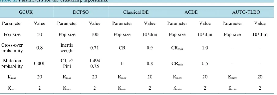
The parameters in cases of all the algorithms are given in Table 1. Where Pop_size indicates the size of the population, dim implies the dimension of each chromosome, and Pini is a user-specified probability used for initializing the position of a particle in the DCPSO algorithm.
4.2. Datasets Used
The following real-life data sets are used in this paper which are taken from [2] [12]. Here, n is the number of data points, d is the number of features, and K is the number of clusters.
1) Iris plants database (n = 150, d = 4, K = 3): This is a well-known database with 4 inputs, 3 classes, and 150 data vectors. The data set consists of three different species of iris flower: Iris setosa, Iris virginica, and Iris ver- sicolour. For each species, 50 samples with four features each (sepal length, sepal width, petal length, and petal width) were collected. The number of objects that belong to each cluster is 50.
2) Glass (n = 214, d = 9, K = 6): The data were sampled from six different types of glass: 1) building win- dows float processed (70 objects); 2) building windows non-float processed (76 objects); 3) vehicle windows float processed (17 objects); 4) containers (13 objects); 5) tableware (9 objects); and 6) headlamps (29 objects). Each type has nine features: 1) refractive index; 2) sodium; 3) magnesium; 4) aluminum; 5) silicon; 6) potas- sium; 7) calcium; 8) barium; and 9) iron.
[image:6.595.91.544.565.721.2]3) Wisconsin breast cancer data set (n = 683, d = 9, K = 2): The Wisconsin breast cancer database contains nine relevant features: 1) clump thickness; 2) cell size uniformity; 3) cell shape uniformity; 4) marginal adhesion; 5) single epithelial cell size; 6) bare nuclei; 7) bland chromatin; 8) normal nucleoli; and 9) mitoses. The data set
Table 1. Parameters for the clustering algorithms.
GCUK DCPSO Classical DE ACDE AUTO-TLBO
Parameter Value Parameter Value Parameter Value Parameter Value Parameter Value
Pop-size 50 Pop-size 100 Pop-size 10*dim Pop-size 10*dim Pop-size 10*dim
Cross-over probability 0.8
Inertia
weight 0.71 CR 0.9 CRmax 1.0 - -
Mutation
probability 0.001
C1, c2 Pini
1.494
0.75 F 0.8 CRmin 0.5 - -
Kmax 20 Kmax 20 Kmax 20 Kmax 20 Kmax 20
has two classes. The objective is to classify each data vector into benign (239 objects) or malignant tumors (444 objects).
4) Wine (n = 178, d = 13, K = 3): This is a classification problem with “well-behaved” class structures. There are 13 features, three classes, and 178 data vectors.
5) Vowel data set (n = 871, d = 3, K = 6): This data set consists of 871 Indian Telugu vowel sounds. The data set has three features, namely F1, F2, and F3, corresponding to the first, second and, third vowel frequencies, and six overlapping classes {d (72 objects), a (89 objects), i (172 objects), u (151 objects), e (207 objects), o (180 objects)}.
4.3. Population Initialization
For all the algorithms, we randomly initialize the activation thresholds (control genes) within [0 and 1]. The cluster centroids are also randomly fixed between Xmax and Xmin, which denote the maximum and minimum numerical values of any feature of the data set under test, respectively.
4.4. Simulation Strategy
In this paper, while comparing the performance of AUTO-TLBO algorithm with other clustering techniques, we focus on two major issues: as 1) ability to find the optimal number of clusters; and 2) computational time re- quired to find the solution. For comparing the speed of the algorithms, the first thing we require is a fair time measurement. The number of iterations or generations cannot be accepted as a time measure since the algo- rithms perform different amount of works in their inner loops, and they have different population sizes. Hence, we choose the number of fitness function evaluations (FEs) as a measure of computation time instead of genera- tions or iterations. Since the algorithms are stochastic in nature, the results of two successive runs usually do not match. Hence, we have taken 40 independent runs (with different seeds of the random number generator) of TLBO algorithm and for others we have directly taken from paper [13]. The results have been stated in terms of the mean values and standard deviations over the 40 runs in each case. As the hierarchical agglomerative algo- rithm “average-link” used here does not use any evolutionary technique, the number of FEs is not relevant to this method. This algorithm is supplied with the correct number of clusters for each problem, and we used the Ward updating formula [18] to efficiently re-compute the cluster distances. We used unpaired t-tests to compare the means of the results produced by the best and the second best algorithms. The unpaired t-test assumes that the data have been sampled from a normally distributed population. From the concepts of the central limit theo- rem, one may note that as sample sizes increase, the sampling distribution of the mean approaches a normal dis- tribution regardless of the shape of the original population. A sample size around 40 allows the normality as- sumptions conducive for performing the unpaired t-tests [16].
Finally, we would like to point out that all the experiment codes are implemented in MATLAB. The experi- ments are conducted on a Pentium 4, 1 GB memory desktop in Windows 7 environment.
4.5. Experimental Results
To judge the accuracy of the clustering algorithms, we let each of them run for a very long time over every benchmark data set, until the number of FEs exceeded 106. Then, we note the number of clusters found and their corresponding CS measure value which is given in terms of means and standard deviation in Table 2.
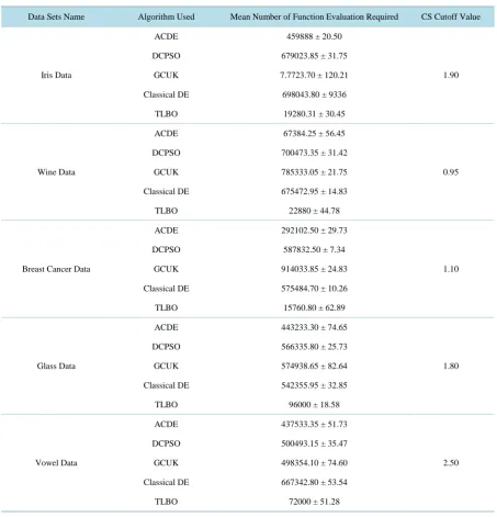
To compare the speeds of different algorithms, we selected a threshold value of CS measure for each of the data sets. This cutoff CS value is somewhat larger than the minimum CS value found by each algorithm in Ta- ble 3. Now, we run a clustering algorithm on each data set and stop as soon as the algorithm achieves the proper number of clusters, as well as the CS cutoff value. We then note down the number of fitness FEs that the algo- rithm takes to yield the cutoff CS value. A lower number of FEs corresponds to a faster algorithm. Table 4
shows results of unpaired t-tests taken on the basis of the CS measure between the best two algorithms (standard error of difference of the two means, 95% confidence interval of this difference, the t value, and the two tailed P value). For all the cases in Table 4, sample size = 40.
4.6. Discussion on Results
Table 2. Final solution (mean and standard deviation over 40 independent runs) after each algorithm was terminated after running for 106 FEs, with CS-measure-based fitness function.
Data Sets Name Algorithm Used Mean and Standard Deviation of Number of Cluster
Mean and Standard Deviation of CS Measure
Exact Cluster Number for Dataset
Iris Data
ACDE 3.25 ± 0.0382 0.6643 ± 0.097
3 DCPSO 2.23 ± 0.443 0.7361 ± 0.671
GCUK 2.35 ± 0.0958 0.7282 ± 2.003
Classical DE 2.50 ± 0.0473 0.7633 ± 0.039
TLBO 3.033 ± 0.3198 0.5014 ± 0.143
Average-Link 3.00 0.7863 ± 0.00
Wine Data
ACDE 3.25 ± 0.0391 0.9249 ± 0.032
3 DCPSO 3.05 ± 0.0352 1.8721 ± 0.037
GCUK 2.95 ± 0.0112 1.5842 ± 0.328
Classical DE 3.50 ± 0.0143 1.7964 ± 0.802
TLBO 3.200 ± 0.0665 0.8848 ± 95
Average-link 3.00 1.8921 ± 0.00
Breast Cancer Data
ACDE 2.00 ± 0.00 0.4532 ± 0.034
2 DCPSO 2.25 ± 0.0632 0.4854 ± 0.009
GCUK 2.00 ± 0.0083 0.6089 ± 0.016
Classical DE 2.25 ± 0.0261 0.8984 ± 0.381
TLBO 2.000 ± 0.00 0.3982 ± 0.098
Average-Link 2.00 0.9007 ± 0.00
Glass Data
ACDE 6.05 ± 0.0148 0.3324 ± 0.487
6 DCPSO 5.95 ± 0.0093 0.7642 ± 0.073
GCUK 5.85 ± 0.0346 1.4743 ± 0.236
Classical DE 5.60 ± 0.0754 0.7782 ± 0.643
TLBO 6.00 ± 0.5872 0.2999 ± 0.511
Average-Link 6.00 1.0221 ± 0.00
Vowel Data
ACDE 5.75 ± 0.0751 0.9089 ± 0.051
6 DCPSO 7.25 ± 0.0183 1.1827 ± 0.431
GCUK 5.05 ± 0.0075 1.9978 ± 0.966
Classical DE 7.50 ± 0.0569 1.0844 ± 0.067
TLBO 5.998 ± 0.7226 0.8595 ± 0.112
Table 3. Mean and standard deviations of the number of fitness FEs (over 40 independent runs) required by each algorithm to reach a predefined cutoff value of the CS validity index.
Data Sets Name Algorithm Used Mean Number of Function Evaluation Required CS Cutoff Value
Iris Data
ACDE 459888 ± 20.50
1.90 DCPSO 679023.85 ± 31.75
GCUK 7.7723.70 ± 120.21
Classical DE 698043.80 ± 9336
TLBO 19280.31 ± 30.45
Wine Data
ACDE 67384.25 ± 56.45
0.95 DCPSO 700473.35 ± 31.42
GCUK 785333.05 ± 21.75
Classical DE 675472.95 ± 14.83
TLBO 22880 ± 44.78
Breast Cancer Data
ACDE 292102.50 ± 29.73
1.10 DCPSO 587832.50 ± 7.34
GCUK 914033.85 ± 24.83
Classical DE 575484.70 ± 10.26
TLBO 15760.80 ± 62.89
Glass Data
ACDE 443233.30 ± 74.65
1.80 DCPSO 566335.80 ± 25.73
GCUK 574938.65 ± 82.64
Classical DE 542355.95 ± 32.85
TLBO 96000 ± 18.58
Vowel Data
ACDE 437533.35 ± 51.73
2.50 DCPSO 500493.15 ± 35.47
GCUK 498354.10 ± 74.60
Classical DE 667342.80 ± 53.54
TLBO 72000 ± 51.28
Table 4. Results of the unpaired t-test between the best and the 2nd best performing algorithm
Dataset Standard Error T 95% Confidence Interval Two-Tailed P Significance
Iris 0.027 5.9624 From −0.217292 to −0.108508 <0.0001 Extremely Significant
Wine 0.012 3.4157 From −0.063472 to −0.016728 0.0010 Very Significant
Breast Cancer Data 0.0012 3.3534 From −0.087652 to −0.022348 0.0012 Very Significant
Glass 0.112 0.2912 From −0.254703 to 0.189703 0.7717 Not Significant
[image:9.595.89.537.602.720.2]but also converges faster in comparison to other algorithms.
5. Conclusion
An important feature of the AUTO-TLBO is that it is able to automatically find the optimal number of clusters (i.e., the number of clusters does not have to be known in advance) like other algorithms and does so in fast convergence time. The AUTO-TLBO algorithm is able to outperform then other five clustering algorithms in a statistically meaningful way over a majority of the benchmark data sets discussed here. This certainly does not lead us to claim that always AUTO-TLBO may outperform other algorithms over every data set since it is im-possible to model all the im-possible complexities of real-life data with the limited test suit that we used for testing the algorithms. In addition, the performance of other algorithm may also be enhanced with a parameter tuning.
References
[1] Jain, A.K., Murty, M.N. and Flynn, P.J. (1999) Data Clustering: A Review. ACM Computing Surveys, 31, 264-323.
http://dx.doi.org/10.1145/331499.331504
[2] Chou, C.H., Su, M.C. and Lai, E. (2004) A New Cluster Validity Measure and Its Application to Image Compression.
Pattern Analysis and Applications, 7, 205-220. http://dx.doi.org/10.1007/s10044-004-0218-1
[3] Storn, R. and Price, K. (1997) Differential Evolution—A Simple and Efficient Heuristic for Globaloptimization over Continuous spaces. Journal of Global Optimization, 11, 341-359. http://dx.doi.org/10.1023/A:1008202821328
[4] Das, S., Abraham, A. and Konar, A. (2008) Automatic Clustering Using an Improved Differential Evolution Algorithm.
IEEE Transactions on Systems, Man, and Cybernetics—Part A: Systems and Humans, 38, 218-237.
[5] Day, W.H. and Edelsbrunner, H. (1984) Efficient Algorithms for Agglomerative Hierarchical Clustering Methods.
Journal of Classification, 1, 1-24. http://dx.doi.org/10.1007/BF01890115
[6] Bandyopadhyay, S. and Maulik, U. (2002) Genetic Clustering for Automatic Evolution of Clusters and Application to Image Classification. Pattern Recognition, 35, 1197-1208. http://dx.doi.org/10.1016/S0031-3203(01)00108-X
[7] Omran, M., Salman, A. and Engelbrecht, A. (2005) Dynamic Clustering Using Particle Swarm Optimization with Ap-plication in Unsupervised Image Classification. Proceedings of the 5th World Enformatika Conference (ICCI), Prague. [8] Clerc, M. and Kennedy, J. (2002) The Particle Swarm-Explosion, Stability and Convergence in a Multi-Dimensional
Complex Space.IEEE Transactions on Evolutionary Computation, 6, 58-72.
[9] Kennedy, J., Eberhart, R.C. and Shi, Y. (2001) Swarm Intelligence. Morgan Kaufmann Publishers, San Francisco.
[10] Blake, C., Keough, E. and Merz, C.J. (1998) UCI Repository of Machine Learning Database.
http://www.ics.uci.edu/~mlearn/MLrepository.html
[11] Raghavan, V.V., Birchand, K., Paterlinia, S. and Krink, T. (2006) Differential Evolution and Particle Swarm Optimiza-tion in PartiOptimiza-tional Clustering. Computational Statistics & Data Analysis, 50, 1220-1247.
http://dx.doi.org/10.1016/j.csda.2004.12.004
[12] Pal, S.K. and Majumder, D.D. (1977) Fuzzy Sets and Decision Making Approaches in Vowel and Speaker Recognition.
IEEE Transactions on Systems, Man, and Cybernetics, 7, 625-629.
[13] Satapathy, S.C. and Naik, A. (2011) Data Clustering Based on Teaching Learning Based Optimization. Lecture Notes in Computer Science, 7077, 148-156.
[14] Murty Ramakrishna, M., Murthy, J.V.R., Prasad Reddy, P.V.G.D., Naik, A. and Satapathy, S.C. (2013) Performance of Teaching Learning Based Optimization Algorithm with Various Teaching Factor Values for Solving Optimization Problems. Proceedings of the International Conference on Frontiers of Intelligent Computing: Theory and Applica-tions (FICTA) 2013, Advances in Intelligent Systems and Computing, 247, 207-216.
[15] Rao, R.V., Savsani, V.J. and Vakharia, D.P. (2011) Teaching-Learning-Based Optimization: A Novel Method for Con- strained Mechanical Design Optimization Problems. Computer-Aided Design, 43, 303-315.
http://dx.doi.org/10.1016/j.cad.2010.12.015
[16] Flury, B. (1997) A First Course in Multivariate Statistics. Springer-Verlag, Berlin.
http://dx.doi.org/10.1007/978-1-4757-2765-4
[17] Omran, M., Engelbrecht, A. and Salman, A. (2005) Particle Swarm Optimization Method for Image Clustering. Inter-national Journal of Pattern Recognition and Artificial Intelligence, 19, 297-322.
[18] Olson, C. (1995) Parallel Algorithms for Hierarchical Clustering. Parallel Computing, 21, 1313-1325.