A predictor corrector iterative method for solving linear least squares problems and perturbation error analysis

R E S E A R C H

Open Access

A predictor-corrector iterative method for

solving linear least squares problems

and perturbation error analysis

Suzan C. Buranay

_{and Ovgu C. Iyikal}

*_{Correspondence:} [email protected] 1_{Department of Mathematics,}

Faculty of Arts and Sciences, Eastern Mediterranean University, Famagusta, North Cyprus, Turkey

Abstract

The motivation of the present work concerns two objectives. Firstly, a

predictor-corrector iterative method of convergence orderp= 45 requiring 10 matrix by matrix multiplications per iteration is proposed for computing the Moore–Penrose inverse of a nonzero matrix of rank =r. Convergence and a priori error analysis of the proposed method are given. Secondly, the numerical solution to the general linear least squares problems by an algorithm using the proposed method and the

perturbation error analysis are provided. Furthermore, experiments are conducted on the ill-posed problem of one-dimensional image restoration and on some test problems from Harwell–Boeing collection. Obtained numerical results show the applicability, stability, and the estimated order of convergence of the proposed method.

MSC: Primary 65F20; secondary 65F30

Keywords: Linear least squares problems; Perturbation error analysis; Moore–Penrose inverse; Image restoration problem; Matrix algorithms

1 Introduction

The numerical solution of many problems in mathematical physics requires the solution of an algebraic linear system of equations. When the coefficient matrix of a consistent linear system is singular or rectangular matrix, then the need for Moore–Penrose inverse occurs for the computation of minimum norm least squares solution.

LetCn1×n2 _andCn1×n2

r denote the sets of all complexn1×n2matrices and all complex n1×n2matrices ofrank=r, respectively. ByA∗,R(A), andPR(A)we present the conjugate transpose ofA, range ofA, and the orthogonal projector ontoR(A) respectively, and as usualIdenotes the unit matrix of appropriate order. The generalized inverse or Moore– Penrose inverse of a matrixA∈Cn1×n2 _{denoted byA}†∈Cn2×n1_{is the unique matrix}

sat-isfying the following four Penrose equations (see [1]):

AA†A=A, A†AA†=A†, AA†∗=AA†, A†A∗=A†A. (1.1)

Many important approaches for computing the Moore–Penrose generalized inversion have been developed. Among these methods, direct methods usually tend to require a pre-dictable amount of resources in terms of time and storage, which normally puts them out

of interest especially for large scaled systems with sparse matrices. Special interest is given to propose and investigate iterative methods for computing the Moore–Penrose inverse A†_{. LetA∈C}n1×n2

r , we survey on iterative methods by whichVmdenotes the approximate

Moore–Penrose inverse ofAat themth iteration, andMmsstands for the matrix by matrix multiplications per iteration. The authors of [2] proposed the sequence

Vm=α m

i=0

A∗I–αAA∗i, m= 0, 1, . . . , (1.2)

that converges toA†_{asm→ ∞under the assumption}

0 <α< 2

λ1(A∗A)

, (1.3)

where

λ1

A∗A≥λ2

A∗A≥ · · · ≥λr

A∗A> 0 (1.4)

are the nonzero eigenvalues ofA∗A. Later in [3] (see also [4]) the iterative method (1.2) was written as follows:

V0=αA∗, (1.5)

Vm+1=Vm+α(I–VmA)A∗, m= 0, 1, . . . , (1.6)

and it converges toA†_{linearly. The following iterative algorithm [5,6]}

V0=αA∗,

Vm+1=Vm(2I–AVm), m= 0, 1, . . . ,

(1.7)

yieldsA†_{as the limit of the sequence{V}

m},m= 0, 1, . . . , whenαsatisfies (1.3). This method

is a variant of the well-known Schulz method of 2nd order. Apth order iterative method for computingA†_{is studied in [7] and [8] forp≥2 andpbeing integer as follows:}

V0=αA∗,

Tm=I–VmA,

Pm= p–1

i=0 Ti_m,

Vm+1=PmVm= _p–1

i=0 Ti_m

Vm, m= 0, 1, . . . .

(1.8)

Method (1.8) is also called hyperpower iterative method and forn1≤n2is usually pre-sented as

Vm+1=Vm p–1

j=0

whereTm=I–AVm, performingp Mms. In [7], whenp= 3, method (1.9) is rewritten in

the form

Vm+1=Vm

3I– 3AVm+ (AVm)2

, m= 0, 1, . . . , (1.10)

and in Horner’s form for the inversion of a square nonsingular matrix is given in [9] as

Vm+1=Vm

3I–AVm(3I–AVm)

, m= 0, 1, . . . , (1.11)

and has at least third order of convergence [7,10]. There are different representations of the hyperpower method (1.9) which differ in the evaluation of the power sump_j=0–1Tmj.

The computational effort in thepth order method decreases when the number of matrix by matrix multiplications and additions in the polynomial are reduced through factoriza-tions if nested loops are used (see [11] and [12]). Whenp= 5, an effective form of the hyperpower iterative method for inverse of a square nonsingular matrix is presented in [11] as follows:

Vm+1=Vm

I+I+T_m2Tm+Tm2

, m= 0, 1, . . . , (1.12)

and requires 4 Mms. To compute the inner inverse of matrixA∈Cn1×n2_{, the following}

iterative procedure is proposed in [13]:

Vm+1=Vm

pI–p(p– 1)

2 AVm+· · ·+ (–1)

p–1_(AV

m)p–1 , p≥2, (1.13)

m= 0, 1, 2, . . . , which requiresp Mms. Equation (1.13) is an equivalent form of (1.9). In [14] the authors showed that the iterative procedure (1.13) can be used to compute the Moore–Penrose inverse of a matrix. The authors of [15] proved that the sequences (1.13) indeed are convergent to a fixed inner inverse of the matrix which is the Moore–Penrose inverse of the matrix, and they provided numerical results for the third order iterations. The following 7th order method is given by [16] for computing generalized inverseA(2)_T,S:

Vm+1=Vm

I+Tm+Tm4

I+Tm+Tm2

, m= 0, 1, . . . . (1.14)

The method in (1.14) performs 5Mms. Recently several systematic algorithms for fac-torizations of the hyperpower iterative family (1.9) of arbitrary orders have been given in [17] for computing outer inverses. Among these methods the 11th, 15th, and 19th order methods are

Vm+1=Vm

I+Tm

I+Tm+Tm2 +Tm3

I+T_m3 +T_m6, m= 0, 1, . . . . (1.15)

Vm+1=Vm

I+Tm+Tm2

I+T_m2 +T_m4I+T_m4 +T_m8, m= 0, 1, . . . (1.16)

Vm+1=Vm

I+Tm+Tm2

I+T_m2 +T_m4I+T_m6 +T_m12, m= 0, 1, . . . , (1.17)

given that each uses 7, 7, and 8Mms, respectively.

to construct inverse preconditioners for solving linear systems. Class 1 methods converge with order of convergencep= 3∗2k_{+ 1 and Class 2 methods converge with order p=}

5∗2k_{– 1, requiring 2k+ 4Mmsand 3k+ 4Mms, respectively. Most recently, high order}

iterative methods with a recurrence formula for approximate matrix inversion have been proposed in [19] with orders of convergencep= 4k+ 3, wherek≥1 is an integer requiring k+ 4 matrix multiplications per iteration. The methods of ordersp= 7, 11, 15, 19 are used to construct approximate Schur-block incomplete LU preconditioners (Schur-BILU) for regularized solution of discrete ill-posed problems.

The original contribution of this study is the construction of a predictor-corrector iter-ative method (PCIM) of convergence orderp= 45 requiring 10Mmsfor computing the Moore–Penrose inverse of nonzero matrixA∈Cn1×n2

r . Also, perturbation error analysis

of the proposed method for the minimum norm solution of least squares problems is pro-vided. To verify the theoretical results, experimental analysis are conducted for the one-dimensional image restoration problem and for some well-conditioned and moderately ill-conditioned problems from Harwell–Boeing collection. Next, a benchmark example is used to numerically compute the order of convergence of the proposed method. Conclud-ing remarks are given in the last section.

Some versions of the predictor-corrector variational iteration method for the solution of integral equations of fractional order were studied in [20] and [21].

2 A predictor-corrector iterative method for approximate Moore–Penrose inverse

LetIdenote then1×n1unit matrix and letA∈Cnr1×n2 and the nonzero eigenvalues of

A∗Abe denoted by (1.4). We define the following matrix-valued functions consisting of matrix multiplications and additions:

Ω(Tm) =Tm+Tm2, (2.1)

Ψ(Tm) =I+Tm2, (2.2)

Γ(Tm) =Tm4, (2.3)

whereTm= (I–AVm). We propose the following:

Predictor-corrector iterative method (PCIM).

In:V0=αA∗

G:Tm=I–AVm, Φ(Tm) =Ψ(Tm)Ω(Tm)

P:V_m+1 2 =Vm

I+Φ(Tm)

, T_m+1

2 =I–AVm+12

C:Vm+1=Vm+1₂

I+Φ(T_m+1 2)

I+Γ(T_m+1 2)

form= 0, 1, 2, . . . . (2.4)

the following form of (2.4) which requiresPR(A):

In:V0=αA∗,

G:Rm=PR(A)–AVm, Φ(Rm) =Ψ(Rm)Ω(Rm),

P:V_m+1 2 =Vm

PR(A)+Φ(Rm)

, R_m+1

2 =PR(A)–AVm+12,

C:Vm+1=Vm+1₂

PR(A)+Φ(Rm+1₂)

I+Γ(R_m+1 2)

form= 0, 1, 2, . . . (2.5)

Lemma 2.1 Let A∈Cn1×n2

r ,if in the initial step In of(2.5α satisfies(1.3),then for the

sequence{Vm+1}obtained at m+ 1th iteration by PCIM(2.5)the following hold true for every m= 0, 1, 2, . . . :

(i) Vm+1PR(A)=Vm+1, (ii) PR(A∗)Vm+1=Vm+1, (2.6)

(iii) (AVm+1)∗=AVm+1, (iv) (Vm+1A)∗=Vm+1A. (2.7)

Proof The proof follows from PCIM (2.5) using mathematical induction. We give the proof of (i) and (iii) and the proof of (ii) and (iv) can be given analogously. By (III) of The-orem 1 [7],AA†=PR(A)andA†A=PR(A∗), and on the basis of Moore–Penrose equations (1.1), the projectionPR(A)satisfies the following:

P2_R(A)=PR(A), P∗R(A)=PR(A), PR(A)A=A; A∗PR(A)=A∗. (2.8)

(i) Form= 0, in the initial stepInof PCIM (2.5) we haveV0=αA∗implyingV0PR(A)=

αA∗PR(A)=αA∗=V0. Assume thatVmPR(A)=Vmholds true form, then using (2.8) for the

predictor stepPof (2.5) we obtain

V_m+1

2PR(A)=Vm

PR(A)+Φ(Rm)

PR(A)

=Vm

PR(A)+ (PR(A)–AVm) + (PR(A)–AVm)2+ (PR(A)–AVm)3

+ (PR(A)–AVm)4

PR(A)=Vm+1₂, (2.9) R_m+1

2 =PR(A)–AVm+12 =PR(A)–AVm

PR(A)+Φ(Rm)

=PR(A)–AVm

PR(A)+Rm+R2m+R3m+R4m

=R5_m. (2.10)

Also in the corrector stepCof (2.5) using (2.10) we get

Γ(R_m+1 2) =R

4

m+1₂ =R 20

m, (2.11)

Φ(R_m+1

2) =Ψ(Rm+12)Ω(Rm+12) =

I+R10_mR5_m+R10_m. (2.12)

Using (2.8) and from the assumptionVmPR(A)=Vm, equations (2.11) and (2.12) imply

Γ(R_m+1

2)PR(A)= (PR(A)–AVm)

20_P

R(A)=Γ(Rm+1₂), (2.13)

Φ(R_m+1 2)PR(A)=

Using (2.8)–(2.14) in the corrector stepCof (2.5), we obtain

Vm+1PR(A)=Vm+1₂

PR(A)+Φ(Rm+1₂)

I+Γ(R_m+1 2)

PR(A)

=V_m+1 2

PR(A)+Φ(Rm+1₂)PR(A)+Φ(Rm+1₂)Γ(Rm+1₂)PR(A)

=V_m+1 2

PR(A)+Φ(R_m+1 2)

I+Γ(R_m+1 2)

=Vm+1. (2.15)

(iii) Form= 0, in the initial stepInof PCIM (2.5) we haveV0=αA∗ implying (AV0)∗= (AαA∗)∗=αAA∗=AV0. Assume that (AVm)∗=AVmholds true, then from (2.8) in the

pre-dictor stepPof (2.5) gives

R∗_m= (PR(A)–AVm)∗=Rm, (2.16)

Φ∗(Rm) =

I+R10_mR5_m+R10_m∗=Φ(Rm), (2.17)

(AV_m+1 2)

∗_=P∗

R(A)+Φ∗(Rm)

(AVm)∗=AVm+1₂. (2.18) From the assumption and also using (2.8), (2.10)–(2.12), and (2.16) gives

R∗_m+1 2 =Rm+

1 2, Γ

∗_(R

m+1₂) =Γ(Rm+1₂), Φ∗(Rm+1₂) =Φ(Rm+1₂). (2.19) Using (2.8), (2.18), and (2.19) in the corrector stepCof (2.5) yields

(AVm+1)∗=

PR(A)+Φ(Rm+1₂)

I+Γ(R_m+1 2)

∗

(AV_m+1 2)

∗

=AVm+1. (2.20)

Remark2.2 The validity of (2.6) and (2.7) for PCIM (2.5) implies that PCIM (2.4) is derived from PCIM (2.5). The computational significance of method (2.5) is limited by the need for knowledge ofPR(A).Therefore, the PCIM given in (2.4) is more effective in computational aspects and is preferable forn1≤n2. Ifn1>n2, then the dual version of PCIM (2.4) can be used.

Theorem 2.3 Let A∈Cn1×n2

r ,if in the initial step In of PCIM(2.4)αsatisfies(1.3),then

the sequence{Vm+1}obtained by the proposed PCIM(2.4)converges to the Moore–Penrose inverse A† _{uniformly with p= 45order of convergence and with asymptotic convergence}

factor[18]ACF=_ln10₄₅≈2.627.Furthermore,the following error estimate is valid:

A†–Vm+1₂≤

α R0 45 m+1

2 A∗ 2 1 – R0 2

, (2.21)

where R0=PR(A)–αAA∗.

Proof To show the uniform convergence of{Vm+1}obtained by PCIM (2.4) toA†, we use the approach analogous to the proof of Theorem 3 of [7]. Let us define the residual in the dual version at initial approximation by

Also, for any integers> 0,

T₀sA=ATs₀ (2.23)

and for PCIM (2.4), for its dual version and from Lemma2.1using (2.10)–(2.12) for PCIM (2.5), we obtain the residual error at the (m+ 1)th iteration as

Tm+1=I–AVm+1=Tm45, m= 0, 1, . . . , (2.24)

Tm+1=I–Vm+1A=T 45

m, m= 0, 1, . . . , (2.25)

Rm+1=PR(A)–AVm+1=R45m, m= 0, 1, . . . , (2.26)

respectively. It follows from (2.24)–(2.26) that, for eachm,

AVm+1=I–T45 m+1

0 , Vm+1A=I–T 45m+1

0 , (2.27)

Vm+1AVm+1=Vm+1–T 45m+1

0 Vm+1. (2.28)

From Lemma2.1, equations (2.6), (2.7) and on the basis of Corollary 4 to Theorem 2 and Theorem 1 of [7] the passage to the limit in (2.27) and (2.28) imply the uniform conver-gence

AVm+1→PR(A), Vm+1A→PR(A∗), Vm+1AVm+1→A†. (2.29)

Therefore, the sequence{Vm+1}converges uniformly toA†with orderp= 45. By denoting

V_m+1 2 =Vm+12

I+T_m5+T_m10+T_m15+T_m20+T_m25+T_m30+T_m35, (2.30)

the corrector stepCof (2.4) can be rewritten as

Vm+1=Vm+₂1 +Vm+1₂T 5

m. (2.31)

We denote the error of PCIM (2.4) at the corrector stepCbyEm+1=A†–Vm+1. Next, by using thatA†AA†=A†and from Lemma2.1equations (2.6) and (2.8), we obtain

Em+1–Em+1Rm+1=A†–Vm+1–

A†–Vm+1

(PR(A)–AVm+1)

=Vm+1

AA†–AVm+1

=Vm+1Rm+1. (2.32)

Using (1.3) and on the basis of Theorem 2 of [6], we haveρ(R0) < 1. SinceR0is Hermitian, this givesρ(R0) = R0 2< 1 and using (2.26) and norm properties

Rm+1 2≤ Rm 452 ≤ R0 45 m+1

2 < 1. (2.33)

From (2.32) using second norm gives

Em+1 2≤

Vm+1Rm+1 2 1 – Rm+1 2

(see [7]). By using (2.26), (2.30), and (2.31), it follows that

Vm+1Rm+1=Vm+1R40mR5m

=Vm+1

PR(A)+R5m+R10m +R15m +R20m +R25m +Rm30+R35m +R40m

–Vm+1

PR(A)+R5m+R10m +Rm15+R20m +Rm25+R30m +R35m

R5_m

=Vm+1

PR(A)+R5m+R10m +R15m +R20m +R25m +Rm30+R35m +R40m

–V_m+1 2

PR(A)+R5m+R10m +Rm15+R20m+Rm25+R30m +R35m

–V_m+1 2T

5

m

PR(A)+R5m+R10m +Rm15+R20m +Rm25+R30m+R35m

R5_m

= (Vm+1–Vm+1₂)

PR(A)+R5m+R10m +R15m +R20m

+R25_m+R30_m +R_m35+R40_mR5_m. (2.35)

From equation (2.35) and using PR(A) 2= 1 and second norm, we get

Vm+1Rm+1 2≤ Rm 52

1 + Rm 52+ Rm 102 + Rm 152 + Rm 202 + Rm 252

+ Rm 302 + Rm 352 + Rm 402

Vm+1–Vm+1₂ 2. (2.36) From (2.30) and (2.31) and using thatV_m+1

2P

s

R(A)=Vm+1₂is valid for every positive integer sand also using second norm, it follows that

Vm+1–Vm+1₂ 2=Vm+1₂ +Vm+1₂

T_m5 –I₂

=V_m+1 2T

40

m2≤ Vm+1₂Rm 2 Rm 392 . (2.37) Also, in view of (2.33),

1 – Rm+1 2≥1 – Rm 452 =

1 – Rm 52

1 + Rm 52+ Rm 102 + Rm 152

+ Rm 202 + Rm 252 + Rm 302 + Rm 352 + Rm 402

. (2.38)

From the predictor stepPof (2.4) and using PR(A) 2= 1 and second norm, it follows that

V_m+1

2Rm 2≤ VmRm 2

1 + Rm 2+ Rm 22+ Rm 32+ Rm 42

. (2.39)

Also

1 – Rm 52=

1 – Rm 2

1 + Rm 2+ Rm 22+ Rm 32+ Rm 42

. (2.40)

Using (2.34), (2.36)–(2.40) and by recursion, we obtain the following inequalities yielding (2.21):

A†_–V m+1₂≤

Vm+1Rm+1 2 1 – Rm+1 2 ≤

Rm 442 Vm+1₂Rm 2 1 – Rm 52

≤ Rm 442 VmRm 2 1 – Rm 2

≤ R0 45 m+1

2 V0 2 1 – R0 2

=α R0 45m+1

2 A∗ 2 1 – R0 2

The proposed PCIM (2.4) requires 5Mmsfor the evaluation of the predictor stepPand 5 Mmsfor the corrector stepC. Therefore, total 10Mmsare needed giving the asymptotic convergence factorACF[18] as 10

ln45 ≈2.627.

3 Perturbation error analysis

We consider the minimum norm solution of the linear system of equations

Ax=b, A∈Rn1×n2_,b∈Rn1_{, (3.1)}

whereb∈R(A) andx∈Rn2_{denotes the unknown solutions andrank(A) =r}≤_min(n

1,n2). The general least squares solution of (3.1) or minimum norm least squares solution is the solution of the problem

min

x∈S x 2, S=

x∈Rn2| _Ax–b

2=min

. (3.2)

System (3.2) always has a unique solutionx=A†_{bcalled the pseudoinverse solution [22]. If}

Ais a square nonsingular matrix, thenA†_=A–1_{. The condition number ofAis defined by} κ(A) = A 2 A† 2. Next we consider the following perturbed general least squares prob-lem:

min x∈S x 2,

S=x∈Rn2| _Ax–b

2=min

, (3.3)

whereA=A+∂A,b=b+∂b, andx=A†_{bis called the regularized pseudoinverse solution}

and∂x=x–x,∂τ=τ–τ and the residuals areτ =b–Ax,τ =b–Ax. Also, we take into account the perturbations satisfyingrank(A) =rank(A) =rand ∂A2

A2 ≤εA,

∂b2

b2 ≤εb.

3.1 Algorithm for approximate regularized pseudoinverse solution

Letxm+1,∂=Vm+1bbe the approximate regularized pseudoinverse solution of (3.3), where

Vm+1is the approximate Moore–Penrose inverse ofAobtained by the PCIM given in (2.4) at them+ 1th iteration by using initial approximationV0=αA∗andαsatisfying

0 <α< 2

λ1(A∗A)

, (3.4)

where

λ1A∗A

≥λ2A∗A

≥ · · · ≥λrA∗A> 0 (3.5)

are the nonzero eigenvalues ofA∗A. Hence the residual error at the corresponding step isτm+1=b–Axm+1,∂. Given a predescribed accuracyε> 0, we propose the following

al-gorithm that uses PCIM (2.4) and approximates the regularized pseudoinverse solution

xm+1,∂.

Algorithm A Choose an initial matrixV0=αA∗under the assumption (3.4).

Step 1 Letm= 0. Evaluatex0,∂=V0bandτ0=b–A x0,∂, then calculate τ_b0 2

2 .

Do Step 2–Step 6 until τm 2

Step 2 EvaluateTm=I–AVm.

Step 3 Apply the predictor stepPof PCIM (2.4) to findV_m+1 2.

Step 4 EvaluateT_m+1

2 =I–AVm+12.

Step 5 Apply the corrector stepCof PCIM (2.4) to findVm+1.

Step 6 Evaluatexm+1,∂ =Vm+1b and τm+1 =b –Axm+1,∂ respectively. Then calculate

τm+12

b2 . Letm=m+ 1.

Step 7 If mis the number of iterations performed, thenym=xm,∂ is the approximate

regularized pseudoinverse solution satisfying τm 2

b2 ≤ε.

Theorem 3.1(Theorem 1.4.6 in [22]) Assume thatrank(A) =rank(A) =r and let ∂A2

A2 ≤

εA, ∂_bb₂2 ≤εb.Then,if η=κ(A)εA< 1,the perturbations∂x and∂τ in the least squares

solution x and the residualτ satisfy

∂x 2≤κ (A) 1 –η

εA x 2+εb

b 2 A 2

+εAκ(A) τ 2 A 2

+εAκ(A) x 2, (3.6)

∂τ 2≤εA x 2 A 2+εb b 2+εAκ(A) τ 2. (3.7)

Theorem 3.2 Assume thatrank(A) =rank(A) =r and let ∂A2

A2 ≤εA,

∂b 2

b2 ≤εb.Letxm,∂=

Vmb be the approximate regularized pseudoinverse solution(3.3)obtained by AlgorithmA. Then,ifη=κ(A)εA< 1,the following inequality holds true:

x–xm,∂ 2≤κ (A) 1 –η

εA x 2+εb

b 2 A 2

+εAκ(A) τ 2 A 2

(3.8)

+εAκ(A) x 2+

α(1 +εb) R0 45

m

2 A∗ 2 A 2 x 2 1 – R0 2

,

where x is the pseudoinverse solution(3.2),τ=b–Ax andR0=PR(A)–AV0.

Proof On the basis of Theorem2.3and the inequality in (2.21), and from Theorem3.1, using (3.6), it follows that

x–xm,∂ 2= x–xm,∂+x–x 2≤ x–x 2+ x–xm,∂ 2

= x–x 2+A†b–Vmb₂≤ x–x 2+A†–Vm₂ b 2

≤κ(A)

1 –η

εA x 2+εb b 2 A 2

+εAκ(A) τ 2 A 2

+εAκ(A) x 2

+α R0 45m 2 A∗ 2 1 – R0 2

b 2

≤κ(A)

1 –η

εA x 2+εb

b 2 A 2

+εAκ(A) τ 2 A 2

+εAκ(A) x 2

+α(1 +εb) R0 45m

2 A∗ 2 A 2 x 2 1 – R0 2

.

4 Numerical results

Mathematica program in double precision for Example1 and Example2and with 900 precision for Example3. The tables adopt the following notations:

TCSALis the total solution cost in seconds of AlgorithmA.

TCSSPALis the total solution cost in seconds of AlgorithmAfor successive

perturba-tions.

Example1 (One-dimensional image restoration problem (see [18,23])) In this test prob-lem we consider the first kind Fredholm integral equation

π

2 –π

2

K(θ,ϕ)f(ϕ)dϕ=g(θ), –π 2 ≤θ≤

π

2. (4.1)

The kernelK(θ,ϕ) and the functionf(ϕ) are as follows:

K(θ,ϕ) =

(cosθ+cosϕ)sinω

ω

2

, (4.2)

with

ω=π(sinθ+sinϕ).

f(ϕ) =exp–4(ϕ+ 0.5)2_{+ 2exp–4(ϕ– 0.5)}2_. (4.3)

By taking the quadrature nodesϕj= –π₂ +(j–0.5)_n2 π,j= 1, . . . ,n2, and the pointsθi= –π₂ +

(i–0.5)π

n1 ,i= 1, . . . ,n1, the discretization of (4.1)–(4.3) gives the discrete ill-posed problem

Auh=b. The right-hand side vectorbis calculated by multiplyingAwithu, whereuis

the trace off(ϕ) on the grid pointsϕj,j= 1, . . . ,n2. We apply the proposed AlgorithmA by using successive perturbations to obtain the regularized pseudoinverse solution for the perturbed systems (A+∂A)yk_=b+∂k_{b, where∂A}

i,j= _δ1_ifi=j

0 ifi=j

and∂k_{b= (δ}k_{, . . . ,δ}k₎T_∈Rn1

for different values of the smoothing parameterδ1_{, andδ}k_{= 0.999δ}k–1_{,k= 2,. . . ,6. Lety}k

mk, k= 1, . . . , 6, be the approximate regularized pseudoinverse solution of

min yk_∈Sky

k

2, S

k_=yk_∈Rn2|_(A+∂A)yk_–b+∂k_b

2=min

, (4.4)

obtained by the given AlgorithmAby performingmkiterations for an accuracy of

τ_mk 2

b 2 ≤

5×10–7_{for the corresponding perturbed system. Table1presents the total iteration} num-berm=6_k=1mkperformed, TCSSPALand the relativeL2norm of the errors using Algo-rithmAwhenn1= 400 andn2= 800.

Table 1 TCSSPAL, iteration numbers, relativeL2norm of the errors obtained by AlgorithmAfor

Example1

δ1 _{TCSSPAL m} u–y

1

m1 2

u 2

u–y_m3

3 2

u 2

u–y5_m

5 2

u 2

u–y_m6

6 2

u 2

10–3 _{0.45 10 1.7423E–02 6.2443E–02 1.1128E–01 1.3823E–01}

10–4 _{0.45 10 9.0878E–03 1.4484E–02 2.0965E–02 2.4639E–02}

10–6 _{0.45 10 8.2943E–03 3.1554E–03 3.3861E–03 3.6325E–03}

10–8 _{0.45 10 8.2620E–03 2.8571E–03 3.2967E–04 4.1878E–03}

Example2 (Test problems from Harwell–Boeing collection) The experiments are carried out on nine of the matrices from the Harwell–Boeing test collection (Duff, Grimes, and Lewis, see [22]). The numerical values of the ABB and ASH matrices are random num-bers uniformly distributed in [–1, 1], while WELL and ILLC have their original values. The WELL and ILLC matrices have the same nonzero structure but different numerical values. A set of consistent least squares problems is defined by taking the exact solution to beu= (1, . . . , 1)T_∈Rn2_{, and the right-hand sidebis obtained by multiplying the}

co-efficient matrixAbyu. We apply the proposed AlgorithmAusing the dual version of PCIM for obtaining the regularized pseudoinverse solution for each test problem, where

∂Ai,j= δifi=j

0 ifi=j

and∂b= (δ, . . . ,δ)T_∈Rn1_{for different values of the smoothing parameterδ.}

Letymbe the approximate regularized pseudoinverse solution obtained by the given

Al-gorithmAusing the dual version of PCIM by performingmiterations for an accuracy of

τm 2

b2 ≤ε. Table2presents the test problems, description of the problems, and the size

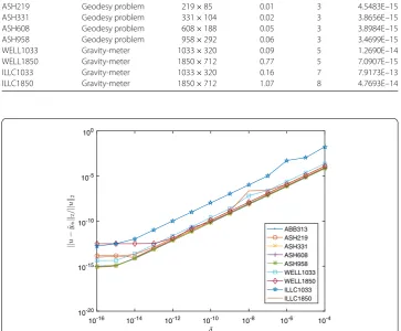
of the matrices, TCSAL, iteration numbersmperformed, and the relativeL2norm of the errors obtained for the test problems in Example2whenδ=ε= 5×10–15_{. Figure1} illus-trates the relativeL2norm of errors for the test problems in Example2with respect toδ. The obtained numerical results justify the theoretical results in Theorem3.2.

Table 2 TCSAL, iteration numbers, and relativeL2norm of the errors obtained by AlgorithmAfor

the test problems of Example2

Test problem Description Size (n1×n2) TCSAL m u–_uym ₂ 2

ABB313 Sudan survey 313×176 0.02 2 3.4674E–15

ASH219 Geodesy problem 219×85 0.01 3 4.5483E–15

ASH331 Geodesy problem 331×104 0.02 3 3.8656E–15

ASH608 Geodesy problem 608×188 0.05 3 3.8984E–15

ASH958 Geodesy problem 958_×292 0.06 3 3.4699E–15

WELL1033 Gravity-meter 1033×320 0.09 5 1.2690E–14

WELL1850 Gravity-meter 1850×712 0.77 5 7.0907E–15

ILLC1033 Gravity-meter 1033×320 0.16 7 7.9173E–13

ILLC1850 Gravity-meter 1850×712 1.07 8 4.7693E–14

Table 3 Second norm errors and the estimated order of convergence of PCIM for Example3

V1–A† 2 V2–A† 2 V3–A† 2 p

0.11199 3.51011E–20 7.43666E–853 47.16

Example3 (A benchmark example [17]) With this example we aim to numerically com-pute the theoretical order of convergence of the proposed PCIM (2.4) using the known exact Moore–Penrose inverse. In this exampleAandA†are

A=

⎛ ⎜ ⎝

1 0 0 –6 2 6 0 –6 7 8 9 –6

⎞ ⎟

⎠, A†=

⎛ ⎜ ⎜ ⎜ ⎝

28 1931

–143 3862

84 1931 –653

3862 1335 7724

–14 1931 57

1931 –249 1931

171 1931 –1903

11,586 –143 23,172

14 1931

⎞ ⎟ ⎟ ⎟ ⎠,

and we use

p=ln

Vm+1–A† 2 Vm–A† 2

ln

Vm–A† 2 Vm–1–A† 2

to estimate the order of convergencep. The maximum norm of the errors and the calcu-lated order of convergencepare presented in Table3. The fourth column of Table3shows that the numerically calculated order of convergencepof PCIM (2.4) is at least 45.

5 Conclusion

The PCIM with convergence orderp= 45 is proposed for computing the Moore–Penrose inverse of a nonzero matrixA∈Cn1×n2

r . Also we give the AlgorithmAwhich uses the

PCIM and approximates the regularized pseudoinverse solution of general least squares problem. The economical computational efficiency and stability of AlgorithmAare useful for the numerical regularized pseudoinverse solution of difficult problems such as the first kind Fredholm integral equations.

Funding Not applicable.

Availability of data and materials

In Example2data are used from “matrix market” a repository organized by the National Institute of Standards and Technology to support this study.

Competing interests

The authors declare that they have no competing interest.

Authors’ contributions

The authors contributed equally to the writing of this paper. All authors read and approved the final manuscript.

Publisher’s Note

Springer Nature remains neutral with regard to jurisdictional claims in published maps and institutional affiliations.

Received: 15 March 2019 Accepted: 9 July 2019 References

1. Penrose, R.: A generalized inverse for matrices. Proc. Camb. Philos. Soc.51, 406–413 (1955)

2. Ben-Israel, A., Charnes, A.: Contributions to the theory of generalized inverses. J. Soc. Ind. Appl. Math.11, 667–699 (1963)

4. Ben-Israel, A., Greville, T.N.E.: Generalized Inverses: Theory and Applications. Springer, Berlin (2003)

5. Ben-Israel, A.: An iterative method for computing the generalized inverse of an arbitrary matrix. Math. Compet.19, 452 (1965)

6. Ben-Israel, A.: A note on an iterative method for generalized inversion of matrices. Math. Compet.20, 439–440 (1966) 7. Petryshyn, W.V.: On generalized inverses and on the uniform convergence of (I–βK)n_{with application to iterative}

methods. J. Math. Anal. Appl.18, 417–439 (1967)

8. Zlobec, S.: On computing the generalized inverse of a linear operator. Glasnik Mat-Fiz. Astronom. Ser. II Drushtvo Mat. Fiz. Hrvatske22, 265–271 (1967)

9. Amat, S., Busquier, S., Gutierrez, J.M.: Geometric constructions of iterative functions to solve nonlinear equations. J. Comput. Appl. Math.157(1), 197–205 (2003)

10. Li, H.-B., Huang, T.-Z., Zhang, Y., Liu, X.-P., Gu, T.-X.: Chebyshev-type methods and preconditioning techniques. Appl. Math. Comput.218(2), 260–270 (2011)

11. Stickel, E.: On a class of high order methods for inverting matrices. Z. Angew. Math. Mech.67(7), 334–336 (1987) 12. Herzberger, J.: Efficient algorithms for the inclusion of the inverse matrix using error-bounds for hyperpower

methods. Computing46, 279–288 (1991)

13. Li, W., Li, Z.: A family of iterative methods for computing the approximate inverse of a square matrix and inner inverse of a non-square matrix. Appl. Math. Comput.215, 3433–3442 (2010)

14. Chen, H., Wang, Y.: A family of higher-order convergent iterative methods for computing the Moore-Penrose inverse. Appl. Math. Comput.218, 4012–4016 (2011)

15. Weiguo, L., Juan, L., Tiantian, Q.: A family of iterative methods for computing Moore-Penrose inverse of a matrix. Linear Algebra Appl.438, 47–56 (2013)

16. Soleymani, F.: An efficient and stable Newton-type iterative method for computing generalized inverseA(2)T,S. Numer.

Algorithms69(3), 569–578 (2015)

17. Soleymani, F., Stanimirovi´c, P.S., Haghani, F.K.: On hyperpower family of iterations for computing outer inverses possessing high efficiencies. Linear Algebra Appl.484, 477–495 (2015)

18. Buranay, S.C., Subasi, D., Iyikal, O.C.: On the two classes of high order convergent methods of approximate inverse preconditioners for solving linear systems. Numer. Linear Algebra Appl.24(6), Article ID e2111 (2017)

19. Buranay, S.C., Iyikal, O.C.: Approximate Schur-block ILU preconditioners for regularized solution of discrete ill-posed problems. Math. Probl. Eng.2019, Article ID 1912535 (2019).https://doi.org/10.1155/2019/1912535

20. Wang, Y.-H., Wu, G.-C., Baleanu, D.: Variational iteration method-a promising technique for constructing equivalent integral equations of fractional order. Cent. Eur. J. Phys.11(10), 1392–1398 (2013)

21. Wu, G.-C., Baleanu, D.: Variational iteration method for the Burgers’ flow with fractional derivatives-new Lagrange multipliers. Appl. Math. Model.37, 6183–6190 (2013)

22. Björck, A.: Numerical Methods for Least Squares Problems. SIAM, Philadelphia (1996)