Mining Massive Datasets

(1)

Mining Massive Datasets

Sakshi khosla

Guru Nanak Dev university, Dept of Computer Science, Gurdaspur

---*---Abstract- The amount of data is increasing at an alarming**

rate. There is a need to adopt different techniques to extract the desired information from the pool of abundant data. The methods of shingling, minhashing and locality sensitive hashing are used to find similar sets. Support vector machine is used for classification and used in the applications of face recognisation.

Keywords:Mining, Map reduce, Shingling, Locality sensitive

hashing, Support vector machine, Face recognisation, Applications

1. INTRODUCTION

Data mining refer to the technique of extracting useful information from large amount of databases. It look for the patterns and data that is not recognized by the summary of data. Data mining is retrieval of hidden and useful information which is retrieved from data warehouses. There are two types of information they are descriptive and predictive information. Descriptive information are those in which patterns are human interpretable and Predictive information find the value of attribute using values of other attributes. Data mining is also called knowledge discovery. It is the process of analyzing data from different perspectives and summarizing it into useful information

1.1 Analysis of data The data is divided into different parts. The analysis is on the basis of class, prediction, cluster and outlier.

1. Class analysis: It include two classes. Data characterization is to summarize the data of class and Data discrimination is the comparison of two classes.

2. Prediction analysis: Prediction is a method which uses the data from the warehouse, and then by using certain algorithms or techniques we come to a conclusion about a specific problem. It is like recommendation system

3. Cluster analysis: It is method of grouping similar type of data in one cluster based on some similarity or other characteristics. An important difference between classification and clustering is that in classification we know the number of classes in advance but in clustering we don’t know the number of classes.

4. Outlier Analysis : It detects the data that do not show general behavior of the data model. Most data mining techniques discard these outliers as being wastage of time to get any useful information from them. But some algorithms consider these outliers or noise or exceptions as an important factor.

1.2 Techniques of data mining

Association is one of the best known data mining

technique. In association, a pattern is discovered based

on a relationship between items in the same

transaction. For example in a retail store it is found

that people buy

potato chips with cold drinks So they put potato chips on sale to promote the sale of cod drinks. Classification is used to classify data into different groups. It uses the technique of decision trees and neural network. A company has to develop a software to predict the number of employees who are going to leave the country. We are using classification technique and divide the employees into two groups .One group consist the name of the employees who are leaving and other who are staying here. The software is used to classify the employees into separate groups.

(2)

2. MAP REDUCE COMPUTATIONAL MODEL

Map reduce is an important concept related to hadoop. Map reduce process vast amounts of data in parallel on large clusters in a reliable and fault tolerant manner. It allows massive scalability across hundreds or thousands of servers in a Hadoop cluster. A MapReduce job usually splits the input data-set into independent chunks which are processed by the map tasks in a completely parallel manner. [2]. The term MapReduce has two separate and distinct tasks that Hadoop programs perform. The first is the map job, which takes a set of data and converts it into another set of data, where individual elements are broken down into tuples (key/value pairs). The reduce job takes the output from a map as input and combines those data tuples into a smaller set of tuples. The reduce job is always performed after the map job.

Fig1:Map Reduce

3. FINDING SIMILAR SETS

To perform the efficient data mining the main aim is to find the similar sets so that a pattern can be formed which can be further used in our model. To find the similar sets we have various techniques .Some of them are briefly described below.

3.1 Shingling of documents: A fundamental data-mining problem is to examine data for “similar” items. The problem of finding textually similar documents can be turned into a set problem by the technique known as “shingling.” The set of unique "shingles" [3] can be used to find similarity of two documents.

3.2 Minhashing: we can use minhashing to compress large documents into small signatures and preserve the expected similarity of any pair of documents,Minhashing compresses large sets in such a way that we can still deduce the similarity of the underlying sets from their compressed versions. It is a technique for quickly estimating how similar two sets are.

[image:2.595.316.534.604.757.2]

3.3 Locality-Sensitive Hashing for Documents: It maps signatures to buckets sothat two similar signatures have a very good chance of appearing in the same bucket. If two signatures are not very similar, they probably don’t appear in one bucket. Then, we only have to compare bucket-mates (candidate pairs ).LSHfocus on the pair of signatures likely to be from the similar documents. In this technique we find the candidate pairs . Candidate pairs are those that hash to the same bucket. we assume that “same bucket” means “identical in some aspect” In this way we get all pairs with similar signatures, but eliminate most pairs that not have similar signatures.

Fig 2: Finding Similar Sets

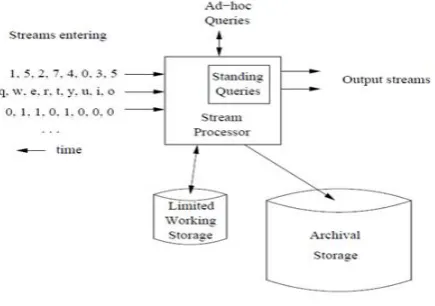
4. MINING DATA STREAMS

A stream processor is a kind of data-management system, the high-level organization [4].Any number of streams can enter the system. Streams may be archived in a large archival store, but we assume it is not possible to answer queries from the archival store. There is also a working store, into which summaries or parts of streams may be placed, and which can be used for answering queries. The working store might be disk, or it might be main memory, depending on how fast we need to process queries. But either way, it is of sufficiently limited capacity that it cannot store all the data from all the streams.

(3)

Rather than deal with an entire data stream, we can think of sampling the stream at periodic intervals. To obtain an unbiased sampling of the data, we need to know the length of the stream in advance. If we do not know this length in advance we need to modify our approach. A technique called reservoir sampling can be used to select an unbiased random sample of s elements without replacement.

4.2 Sliding Windows

Instead of sampling the data stream randomly, we can use the sliding window model to analyze stream data. The basic idea is that rather than running computations on all of the ,we can make decisions based only on recent data. More formally, at every time t, a new data element arrives. This element “expires” at time t +w, where w is the window “size” or length. [5] The sliding window model is useful for stocks or sensor networks, where only recent events may be important. It also reduces memory requirements because only a small window of data is stored.

5. SUPPORT VECTOR MACHINE

5.1 Introduction:-The Support Vector Machine (SVM) is a new and very promising classification technique developed by Vapnik and his group at AT&T Bell Laboratories. The main idea behind the technique is to separate the classes with a surface that maximizes the margin between them. When the data set is large the optimization problem becomes very challenging, because the quadratic form is completely dense and the memory requirements grow. Support Vector Machines are based on the concept of decision planes that define decision boundaries. A decision plane is one that separates between a set of objects having different class memberships. SVM also has concept of underfit and overfit. [6] When the problem is easy to classify and the boundary functions are more complicated than it needs to be the boundary is said to be overfit. When the problem is hard and the classifier is not powerful enough then it is called to be underfit. Another characteristics of SVM is that its boundary function is described by support vectors which are the data located to the closest of its boundary.

Fig4: Support Vector Machine

5.2 Reason to use SVM

Support vector machine have been promising methods for data classification and regression. Their success in practice has been drawn by their solid mathematical foundations which convey several salient properties [7]:

Margin Maximization-The classification boundary functions of SVM maximizes the margin, which in machine learning theory corresponds to maximize the performance. Non Linear transformation of the feature space using kernel trick-SVM efficiently handle non linear classification using the kernel trick which implicitly transform the input space into another high dimensional feature space. The success of SVM in machine learning naturally leads to its possible extension to large scale data mining.

5.3 Problems with SVM for large scale data mining

 Scalability: SVMs are unscalable to data size while common data mining applications often involve millions or billions of data objects.

 Applicability: SVMs are limited to (semi-)supervised learning which is mostly applied to binary classification problems.

 Interpretability: It is hard to interpret and extract knowledge from SVM models.

6. HIERARCHIAL MICRO CLUSTERING

ALGORITHM FOR LARGE DATA SETS

(4)

features) tree, in one scan of the data set given a limited amount of resources by incrementally and dynamically clustering incoming multi dimensional data. The CF tree captures the major distribution patterns of data and provide enough information for CB-SVM to perform. CF tree is a height balanced tree with two parameters : branching factor f and threshold t.

6.2 Algorithm Description

A CF tree is built up dynamically as new data object is inserted. The ways that it inserts a data into same subcluster, merges leaf nodes and manages nonleaf nodes are similar to those in B+ tree.

 Identifying the appropriate leaf: Starting from the root, it descends the CF tree by choosing the child node whose centroid is the closest.

 Modifying the leaf: If the leaf entry can absorb the new data object without violating the threshold conditions, update just the CF vector of the entry. Otherwise add a new entry. If adding a new entry causes a node split, split the node by choosing the farthest pair of entries as seeds and redistributing the remaining entries based on the closeness.  Modifying the path to the leaf: It updates the CF vectors of

each non leaf entry on the path to the leaf. Node split in the leaf causes an insertion of a new non leaf entry into the parent node and if the parent node is split a new entry is inserted into the higher level node. Likewise this occurs recursively to the root. Due to the limited number of entries in a node, a highly skewed input could cause two subclusters that should have been in one cluster split across different nodes and vice versa.

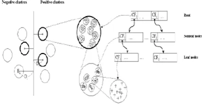
6.3 Clustering Based SVM (CB_SVM)

We present the CB SVM algorithm which trains a very large data set using the hierarchical micro clusters to construct an accurate SVM boundary function. CB-SVM is designed for handling very large data sets. CB-SVM applies a hierarchical micro clustering algorithm that scans the entire dataset only once to provide an SVM with high quality samples. CB-SVM is dependent upon the number of support vectors which is usually much smaller than the entire data. hence it is very scalable for large data sets and leads to high accuracy.

The key idea CB_SVM is to use the hierarchical micro clustering technique to get finer description closer to the boundary and coarser description farther from the

[image:4.595.322.524.253.359.2]

boundary, which can be efficiently accessed as follows: [8] CB_SVM first construct two micro cluster trees called CF tree from positive and negative training data respectively. In each tree a node in higher level is as summarized representation of its children nodes. After constructing the two trees, CB SVM starts training an SVM only from the root nodes. CB SVM is used for classifying very large data sets of relatively low dimensions such as streaming data and data in large warehouses. It performs well for random sampling.

Fig 5: Cluster based SVM

6.4 Summary of the algorithm

1) Construct two CF trees positive and negative data set independently.

2) Train an SVM boundary function using the centroids of the root entities that is the entries in the root node of the two CF trees. If the root node contains too few entities train it using the entries of the nodes at the second leaves of the trees.

3) Decluster the entries near the boundary into the next level and the children entries declusterd from the parent entries are accumulated into the training set with the non declustered parent entries.

4) Construct another SVM from the centroids of the entries in the training set and repeat from step 3 until nothing is accumulated.

6.5 Applications of SVM : Support vector can be used in various real world areas.

 Text and hypertext categorization  Image classification

(5)

7. FACE RECOGNISATION USING SVM

SVM has an important application of fully automatic human face recognizer which usually identify and locate faces in an unknown image. The face detection problem can be defined as follows: Given as input an arbitrary image, which could be a digitized video signal or a scanned photograph, determine whether or not there are any human faces in the image, and if there are, return an encoding of their location. The encoding in this system is to fit each face in a bounding box defined by the image coordinates of the corners.

Some common sources of pattern variations are facial appearance, expression, presence or absence of common structural features, like glasses or a moustache, light source distribution, shadows, etc. The system works by testing candidate image locations for local patterns that appear like faces using a classification procedure that determines whether or not a given local image pattern is a face or not. Therefore, the face detection problem is approached as a classification problem given by examples of 2 classes: faces and non-faces.

7.1 The SVM Face Detection System

This system detects faces by exhaustively scanning an image for face-like patterns at many possible scales, by dividing the original image into overlapping sub-images and classifying them using a SVM to determine the appropriate class, that is, face or non-face. [10]

Clearly, the major use of SVM's is in the classification step, and it constitutes the most critical and important part of this work. It gives a geometrical interpretation of the way SVM's work in the context of face detection. The system works as follows:

1. A database of face and non-face 19*19 pixel patterns, assigned to classes +1 and -1 respectively, is trained on, using the support vector algorithm. A 2nd-degree polynomial kernel function and an upper bound C = 200 are used in this process obtaining a perfect training error.

2. In order to compensate for certain sources of image variation, some preprocessing of the data is performed:

 Masking: A binary pixel mask is used to remove some pixels close to the boundary of the window pattern allowing a reduction in the dimensionality of the input space from 19*19=361 to 283. This step is important in the reduction of background

patterns that introduce unnecessary noise in the training process.

 Illumination gradient correction : A best-fit brightness plane is subtracted from the unmasked window pixel values, allowing reduction of light and heavy shadows

 Histogram equalization: A-histogram equalization is performed over the patterns in order to compensate for differences in illumination brightness, different cameras response curves, etc.

3. Once a decision surface has been obtained through training, the run-time system is used over images that do not contain faces, and misclassifications are stored so they can be used as negative examples in subsequent training phases. [11] Images of landscapes, trees, buildings, rocks, etc., are good sources of false positives due to the many different textured patterns they contain. This bootstrapping step is very important in the context of a face detector that learns from examples because:

 Although negative examples are abundant, negative examples that are useful from a learning point of view are very difficult to characterize and define.  By approaching the problem of face detection, by

using the paradigm of binary pattern classification, the two classes, object and non-object are not equally complex since the non-object class is broader and richer, and therefore needs more examples in order to get an accurate definition that separates it from the object class. Figure shows an image used for bootstrapping with some misclassifications, that were later used as negative examples.

Fig6: SVM separate the face and non face class

4. It performs the following operations:

 Re-scale the input image several times.

(6)

correction and histogram equalization.  Classify the pattern using the SVM.

 If the class corresponds to a face, draw a rectangle around the face in the output image.

7.2 Experimental Results

To test the run-time system, we used two sets of images. The set A, contained 313 high-quality images with same number of faces. The set B, contained 23 images of mixed quality, with a total of 155 faces. Both sets were tested using our system and the one by Sung and Poggio In order to give true meaning to the number of false positives obtained, it is important to state that set A involved 4,669,960 pattern windows, while set B 5,383,682. Table shows a comparison between the 2 systems.

Fig7:Experimental Results

8. FUTURE DIRECTIONS IN FACE DETECTION AND

SVM APPLICATIONS

Future research in SVM application can be divided into three main categories or topics:

1. Simplification of the SVM: One drawback for using SVM in some real-life applications is the large number of arithmetic operations that are necessary to classify a new input vector. The mathematical operations performed are very complex to understand. There is a need of simpler operations while using SVM techniques.

2. Detection of other objects: SVM's is used to detect other objects in digital images, like cars, airplanes, pedestrians, etc. most of these objects have very different appearance, depending on the viewpoint. In the context of face detection, an interesting extension that could lead to better understanding and approach to other problems, is the detection of tilted and rotated faces

3. Use of multiple classifiers: The use of multiple classifiers offers possibilities that can be faster and/or more accurate. The performance can be improved by using multiple classifiers in support vector machines.

9. REFERENCES

[1] m. kaufmann, "data mining concepts and techniques," 2002.

[2] r. a. ulman, "map reduce lecture," in stanford university.

[3] leskovac, "finding similar sets," in stanford university, 2014.

[4] A. Mdatar, "maintaining stream statistics over sliding windows," SIAM J Computing, 2002.

[5] J. G. a. R. R. M Garofalakis, "data stream management," no. springer, 2009.

[6] C. Burges, "tutorial on support vector machine and pattern recognisation," 1998.

[7] V. Vapnik, "Statistical learning theory," no. john wiley and sons, 1998.

[8] R. R. a. M. L. T Zhang, "data clustering method for very large databases," pp. 103-114, 1996.

[9] S. T. a. D. Koller, "support vector machine active learning with applications," no. conference machine learning, p. 990, 2000.

[10] G. B. a. D. carel, "Detection and localization of faces on digital images," p. 967, 1994.

Mining Massive Datasets