Optimization in Genetically Evolved Fuzzy Cognitive Maps Supporting Decision Making: The Limit Cycle Case

Munich Personal RePEc Archive

Optimization in Genetically Evolved

Fuzzy Cognitive Maps Supporting

Decision-Making: The Limit Cycle Case

ANDREOU, A.S. and MATEOU, N.H and Zombanakis,

George A.

University of Cyprus, University of Cyprus, Bank of Greece

19 April 2004

Online at

https://mpra.ub.uni-muenchen.de/51378/

Optimization in Genetically Evolved Fuzzy Cognitive Maps Supporting

Decision-Making: The Limit Cycle Case

A. S. Andreou

*

N. H. Mateou

G. A. Zombanakis

University of Cyprus,

Dept. of Computer Science,

75 Kallipoleos str., CY1678

Nicosia, Cyprus,

[email protected]

University of Cyprus,

Dept. of Computer Science,

75 Kallipoleos str., CY1678

Nicosia, Cyprus

[email protected]

Bank of Greece,

Research Dept.,

21 Panepistimiou str.,

Athens 10250, Greece

[email protected]

* _{Contact author}

Abstract

This paper presents the dynamic behavior of a hybrid system comprising Fuzzy Cognitive Maps and Genetic Algorithms, and focuses on the behavior observed when the system reaches equilibrium at fixed points or limit cycle. More specifically, the present works examines the theoretical background of the equilibrium and limit cycle behaviors and proposes a defuzzification method to handle the latter case. The proposed method calculates the mean value of a limit cycle and uses this value in the defuzzification process along with a confidence rate, which indicates the reliability of the results.

1. Introduction

This paper examines the use of Fuzzy Cognitive Maps (FCMs) as a technique for modeling real-world problems and supporting the decision-making process. More specifically, it focuses on handling the limit cycle phenomenon and proposing an improvement in the decision-making process.

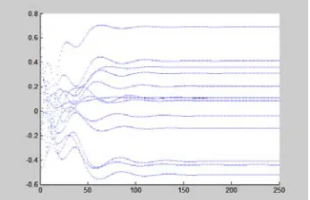
FCMs use notions borrowed from artificial intelligence and neural networks to combine concepts [1, 17] and causal relationships, aiming at creating dynamic models that describe a given cognitive setting [9]. The concepts are represented as nodes, and the causal relationships between these concepts are represented as directed arrows (weights). The development of the FCM is based on the utilization of domain experts’ knowledge that defines the active concepts and the degree of influence between them in the form of numerical values [5]. The activation level of the nodes participating in an FCM model can be calculated using specific updating equations in a series of iterations, after which the model can either reach equilibrium at fixed points in a direct way with activation levels ranging in the interval [-1, 1] (figure 1) or, instead, exhibit a limit cycle behavior (figure 2) [11].

[image:2.595.338.511.327.439.2]

Recently, an enhancement of the classic FCM was introduced [3, 4], which combines FCMs with Genetic Algorithms to facilitate the study of hypothetical scenaria describing the real-world problem under study and provide new and more powerful means for decision-making.

Figure 1. Equilibrium reached by various concepts of an FCM

Figure 2. Limit-cycle reached by various concepts of an FCM

decision-makers are able to introduce hypothetical cases in the model which can be reflected through a target activation level for a certain concept and consider the corresponding weights and activation levels for the rest of the concepts, thus compatible with the predetermined target activation level.

Once the system reaches equilibrium, the decision-makers use this information in order to take decisions leading to the desired simulated solution. In cases, however, in which the system reaches limit cycle decision-making is practically impossible. Once in a simple FCM environment, one approach to overcome this problem is to consult once again with the experts to estimate the external factor which influences one or more concepts and causes the instability of the system. When a GEFCM is used, though, domain experts are not able to help since the weight recalculation is performed with the involvement of Genetic Algorithms (GAs), thus creating a hybrid model. This paper proposes an extension of Genetically Evolved Fuzzy Cognitive Maps (GEFCMs) aiming at increasing their reliability by overcoming the aforementioned weakness appearing in cases of a limit cycle behavior.

2. Genetically Evolved Certainty Neuron

Fuzzy Cognitive Maps

The Fuzzy Cognitive Map (FCM) theory was developed recently [8, 10] as an extension to cognitive maps [2], providing a graphical knowledge representation language that describes a given decision basis in the form of an acyclic graph. The concepts (propositions or states) used by an individual decision-maker, are represented as nodes, while directed arrows denote the causal relationships (interactions) between these concepts. Each arrow is characterized by a weight, a real value that indicates the effect of the causal relationship between nodes. Each concept node possesses a numeric state, which denotes the qualitative measure of its presence in the conceptual domain.

A FCM works in discrete steps [10]. When a strong positive correlation exists between the current state of a concept and that of another concept in a preceding period, we say that the former exercises a positive influence on the latter, this being indicated by a positively weighted arrow directed from the causing to the influenced concept. By contrast, when a strong negative correlation exists, it reveals the existence of a negative causal relationship indicated by an arrow charged with a negative weight. Once the activation levels of the system nodes as well as the weighted arrows are set to a specific value based on experts’ assessment, the system is free to interact [14]. This interaction continues until the model reaches a stable equilibrium, or presents a limit cycle or, even, a chaotic behavior [6].

The introduction of Certainty Neuron Fuzzy Cognitive Maps (CNFCMs) [15] in 1997 provided additional fuzzification to FCMs, by allowing for

various activation levels of each concept between the two extreme cases, i.e. activation or not. More specifically, an updating function f() was used to revise the certainty factor of a concept after receiving new evidence concerning previous beliefs based on the present certainty factor. The updating function of a CNFCM is given in equation (1) as follows:

(

)

t i i t i t i f t

i S A d A

A +1 = − ₍₁₎

where

∑

≠ = = n i j j ij t j t

i A w

S

1 (2)

and Ai is the activation level of concept Ci at

times (t+1) or (t). Equation (2) is the sum of the weighted influences that concept Cireceives at time step

t from all other concepts, di is a decay factor and f() is

the function used for the aggregation of certainty factors [3, 4, 16] :

( )

⎪ ⎪ ⎪ ⎪ ⎪ ⎩ ⎪⎪ ⎪ ⎪ ⎪ ⎨ ⎧ ⎟ ⎟ ⎟ ⎠ ⎞ ⎜ ⎜ ⎜ ⎝ ⎛ ⎟ ⎟ ⎠ ⎞ ⎜ ⎜ ⎝ ⎛ − + ≤ < < − + = + + ≥ ≥ − + = − + = otherwise t i S Ati St_i

At_i

St_i At_i St_i At_i if At_i St_i St_i At_i At_i St_i At_i

St_i At_i if At_i St_i St_i At_i At_i St_i At_i

St_i At_i f m , , min 1 1 | |,| ,| 0 , 0 , ) 1 ( 0 , 0 , ) 1 ( ) , ( (3a) (3b) (3c)

The meaning of equation (3-a,b,c) is that the external influence can affect the activation of a concept just to a certain degree. The activation levels given by the model are related with the values stored in the fuzzy knowledge base yielding the meaning of each concept in terms of output [7].

It is observed that modifications of the weight matrix of the map lead to different dynamic behavior of the system. In the Genetically Evolved Certainty Neuron Fuzzy Cognitive Map (GECNFCM) the optimal weight matrix corresponding to a desired activation level for a given concept is calculated in order to overcome the main weakness of the CNFCM model, namely the need to recalculate the weights corresponding to each concept every time a new strategy is adopted [3, 4]. More specifically, the Genetic Algorithm (GA) [12] evolves a population of individuals, each of which consists of a weight matrix describing the degree of causal relationships between the concepts participating in the map. The activation level of a certain concept in focus denoted by Ad,i is used to calculate the fitness of each

individual-weight matrix WMi according to the

following function:

fitness(WMi)=1/(1-abs(Ad,i –

mean50(Aa,i))

(4)

where Ad,i is the target (desired) value of the

activation level for the concept in focus Ci and

mean50(Aa,i) is the mean value of the last fifty actual

activation levels of concepts Ci as these are computed by

the CNFCM (t variable in equation (3)).

When a GECNFCF hybrid system enters into limit cycle [9] the experts cannot identify the external influences that drive the system to this behavior as in the case of the simple FCM, due to the fact that these influences are controlled automatically by the optimization process of the Genetic Algorithm. Thus, the only alternative is to turn to a method that will attempt to smoothen the limit cycle observed and reliably defuzzify the resulted smoothened value.

3. The Limit Cycle case

A GECNFCM can reach equilibrium at fixed points in a direct way with the activation to be decimals in the interval [-1, 1]. It can also reach a limit cycle behavior in which the system falls in a loop of specific period, and after a certain number of steps, it reaches the same state [18]. A Limit Cycle phenomenon is encountered in cases in which a dynamic system falls into periodic oscillations, failing to reach equilibrium. Oscillations can occur in neural systems due to properties of single neurons [11] and properties of synaptic connectivity among neurons.

The equations that are applied at equilibrium points can be calculated by means of equation (1). For the equilibrium state we have

n i for A

A_it+1_{= i}t, ₌1... ₍₅₎

This is true only when and are of the same sign [15]. In equation (3) the equilibrium point is reached by the use either of the first or the second rule (equation (3a) and (3b) respectively).

t i

A

S

it

When both and take positive values, using the first rule of equation (3), we can calculate the equilibrium value as follows:

t i

A

S

_it

If

A

_it>0 and

S

it>0 then

t i t i i t i t i t i t i t

i

A

A

S

A

d

A

A

A

+1

=

⇒

+

(

1

−

)

−

=

t i t i i t i t i i t i t i t

i

S

A

d

A

A

d

S

S

S

−

−

=

⇒

+

=

⇒

0

(

)

)

(

t i i t i t i

S

d

S

A

+

=

⇒

(6)

When both and take negative values, using the second rule of equation (3) we can calculate the equilibrium value as follows:

t i

A

S

it

If

A

it<0 and <0 then

t i

S

t i t i i t i t i t i t i t

i

A

A

S

A

d

A

A

A

+1

=

⇒

+

(

1

+

)

−

=

t i t i i t i t i i t i t i t

i SA dA A d S S

S + − = ⇒ − =

⇒ 0 ( )

)

(

t i i t i t i

S

d

S

A

−

=

⇒

(7)

In case that and are of opposite signs, using the third rule of equation (3) we can conclude that

cannot be satisfied:

t i

A

S

it

t i t i

A

A

+1

=

t i t i t i t i i t i t i M t i t i t i M t i t i A A A A d S A f A S A f S A < ⇒ < − ⇒ < ⇒ < > +1 ) , ( ) , ( 0 , 0 (8) t i t i t i t i i t i t i M t i t i t i M t i t i A A A A d S A f A S A f S A > ⇒ > − ⇒ > ⇒ > < +1 ) , ( ) , ( 0 , 0 (9)

In the above case ( and of opposite signs) the system enters into limit cycle behavior and values of the various concept activation levels change periodically, something that reveals the existence of strong interactions between the concepts [15].

t i

A

S

_it

3.1 Smoothening and defuzzification

technique for handling limit cycle behavior

The structure of a limit cycle must be first investigated before applying any smoothening technique. The functioning of an oscillation is characterized by three parameters: (i) frequency, (ii) phase and (iii) amplitude [13]. Equilibrium can be described as the case in which all oscillatory units of an ensemble stabilize their frequency to a constant value and their phase and amplitude difference to a constant point within the interval [–1, 1]. The stability of an equilibrium oscillation can be described as follows:

∞ → →Fconst for t t

Fk( ) ,

|Pk(t)−Pk+1(t)|→0,for t→∞ (10) for every k=1,2,...,n−1

where F_k(t)is the frequency of the kth oscillator, at time t in the ensemble of n oscillators, and is its phase at time t.

) (t

Pk

considered as a possible reliable input for inference purposes by the defuzzification process.

Before moving to describing how a limit cycle may be defuzzified based on its Mean value, it is necessary to outline some basic notions of fuzzy sets. The use of fuzzy sets provides a basis for a systematic way of manipulating vague and imprecise concepts and as such they are often treated as representing linguistic variables. A linguistic variable can be regarded either as a variable, the value of which is a fuzzy number, or as a variable assuming valuesdefined in linguistic terms. A linguistic variable may be described by the quintuplet (x, T(x),U, G, M) in which x is the name of variable, T(x) is the term set of x, that is, a set of linguistic values of x each of which corresponds to a fuzzy number defined in a set of real values U, G is a syntactic rule for generating the linguistic of values of x from their numerical counterpart, and M is a semantic rule for associating with each value its meaning [5]. Each term u in T(x) can be classified in a certain fuzzy set A using a membership

function which provides a real number in the interval [0, 1] indicating the degree to which u belongs to set A. A value of 0 means that the term is not a member of the set while a value of unity denotes entire set membership.

] 1 , 0 [ )

( = →

Α u U

µ

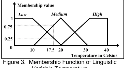
A rather straightforward example will clarify the matter: If we interpret Temperature, for example, as a linguistic variable we may have a term set T(temperature)={Low, Medium, High} and each term in the term set may be characterized by a fuzzy set in a universe of discourse U=[0oC, 40oC]. The three crisp variables may be defined as Low=10o_{C, Medium=20}o_C and High=30oC. This definition, though, does not cover values between the crisp variables, e.g. when temperature ranges between 0oC and 10oC, 10oC and 20oC, 20oC and 30oC. This is the reason why the classical set operations must be extended from ordinary set theory to fuzzy set theory. The values that extend the crisp concepts reduce to their meaning when the fuzzy subsets have membership degrees.For example we may interpret Low as “Temperature below 10o_{C”, Medium as} “Temperature close to 20oC” and High as “Temperature above 30o_{C”. The terms can then be characterized as} fuzzy sets whose membership functions are:

⎪ ⎩ ⎪ ⎨ ⎧

≤ ≤ −

− ≤ =

otherwise

v if v

v if

v Low

, 0

) 20 10 ( , 10 / ) 10 ( 1

10 ,

1 )

( (11)

⎪⎩ ⎪ ⎨

⎧ − − ≤ ≤

=

otherwise

v if v

v Medium

, 0

) 30 10 ( , 20 / 20 1 )

( (12)

⎪ ⎩ ⎪ ⎨ ⎧

≤ ≤ −

− ≥ =

otherwise

v if v

v if

v High

, 0

) 30 20 ( , 10 / ) 30 ( 1

30 ,

1 )

( ₍₁₃₎

[image:5.595.319.534.366.485.2]

The fuzzification of the three crisp values as shown in figure 3 causes the distribution of the variables according to a certain profile that reflects the problem under study. It is obvious that this distribution produces two overlapping areas. Despite the fact, however, that overlapping is both common and even desirable on certain occasions, there is a problem with allocating values that fall within an overlapping area. For example, if temperature is equal to 17.5oC then this temperature belongs to both the Low and the Medium fuzzy sets, with membership values 0.25 and 0.75 respectively. Thus, we may infer that this temperature value maybe considered as low with confidence level 25% and medium with 75%. It is quite important to note in this case that we do not rule out the Low set membership of this temperature value just because its confidence level is significantly lower compared to that of the Medium set. The reason is that the fuzzy interpretation of a linguistic variable within overlapping areas is usually highly subjective. In cases in which this fuzzy structure is used for decision-making, in particular, the two alternative classifications of the linguistic variables are equally important as indicating that more than one approach (decisions) must be taken into consideration.

Figure 3. Membership Function of Linguistic Variable Temperature

Membership value

Medium High Low

1

In Fuzzy Cognitive Maps the term set consists of specific linguistic variables describing the activation levels of the concepts participating in the model. These variables are associated with values within the range [–1, +1]. The number of linguistic variables depends on the complexity of the real-world problem described by the model and the desired model accuracy. The general structure of the fuzzification of the crisp variables describing the activation levels is given in figure 4.

Having described in brief the basic fuzzification notions, we return now to the defuzzification task. The defuzzification process calculates a single numerical value for a fuzzy output variable on the basis of the inferred resulting membership function for this variable. This process, though, becomes extremely difficult when a dynamic system falls into periodic oscillations [9]. We shall attempt to improve inference in this case by attaching a confidence rate to the resulting smoothened activation levels. The reliability of the system may thus be increased and the fault rate decreased. The essence of the proposed defuzzification after performing the smoothening of the limit cycle lies with attaching a

0 0.75

0.25

17.5

10 20 30 40

degree of confidence to the results that will suggest whether the smoothened values found are reliable enough to be used in the decision making process.

[image:6.595.55.296.114.202.2]

Figure 4. Example of fuzzification in the interval [-1, 1]

The proposed defuzzification process for a certain activation level under limit cycle consists of two basic steps:

Step 1. The first step involves classifying the activation level with respect to its Minimum and Maximum values as “BOUNDED LIMIT CYCLE”, or “UNBOUNDED LIMIT CYCLE – POSSIBLE CHAOS”. Since the range of values for the activation levels in our case is [-1, 1] the Baseline Size of the interval is 2. Using the Minimum and Maximum values, we take the difference Diff =(Maximum-Minimum) and calculate the percentage of this value with respect to the baseline size. If Diff is lower or equal to the 75% of the Baseline Size then the oscillation of the activation level is characterized as “BOUNDED LIMIT CYCLE” and inference is possible through the Mean value of step 2: The Mean Value is matched to the appropriate fuzzy interval and defuzzified. Otherwise, (Diff>0,75*Baseline Size) the oscillation is characterized as “UNBOUNDED LIMIT CYCLE – POSSIBLE CHAOS”. In this case the oscillation spans all the available space in the range [Minimum, Maximum] and thus the Mean value cannot be matched to a single fuzzy interval with confidence. Therefore, inference is not possible due to the low degree of reliability of the resulting Mean value.

Step 2. This step is followed only in the case of a “BOUNDED LIMIT CYCLE”. The Mean value of the specific activation level presenting limit cycle is matched with a certain fuzzy set interval according to the analysis given for the specific concept. There are two possibilities here:

(i) Either the Mean value falls in one interval only, and thus the confidence level of belonging to this fuzzy set is 100%, or,

(ii)The Mean value falls between two overlapping fuzzy intervals, thus having two confidence levels, one for each interval. In this case, the confidence levels are calculated as the value of the membership function of the Mean value for each of the overlapping fuzzy intervals. The interval chosen for inference purposes is the one for which the Mean value has the highest membership value, or, equivalently, the highest confidence level.

core core core core core core

Figure 5. Limit Cycle before smoothening

Figure 6. Limit cycle and smoothening

Figures 5 and 6 demonstrate the proposed smoothening method: The system ran for a total of 250 iterations (N variable) presenting limit cycle behavior. After 100 iterations (N’ variable) the smoothening was completed. The Mean value of every activation level presenting limit cycle was first computed and then investigated for proper classification of each oscillation. According to this investigation, all limit cycles were classified as “BOUNDED”. Thus, smoothening was considered as being reliable and for the next 150 iterations (T variable) the system was forced to stabilize and reach equilibrium at the fixed points of the smoothened values. The inference resulted from the defuzzification is out of the scope of this short method demonstration, and has therefore been omitted..

5. Conclusions

This paper proposes an extension of Genetically Evolved Fuzzy Cognitive Maps (GEFCMs), aiming at increasing their reliability by overcoming a significant weakness appearing in cases of a limit cycle. In such a case domain experts are not able to help as the weight recalculation is performed with the involvement of Genetic Algorithms (GAs).

The proposed method for handling the limit cycle case is divided into two parts: The first part calculates the mean value of the limit cycle oscillation of every activation level participating in the conceptual domain. The mean value of each activation level is considered as the equilibrium point of the corresponding smoothened limit cycle. The second part investigates the structure of a certain limit cycle and attaches a degree of confidence to the output suggesting whether the resulting smoothened activation level value is reliable enough to

a2 b1

a1=-1 a3 b2 b(n

a(n/2)+2 a(n/2)+3

b(n/2+2)

an

… … _{bn-1 b}

[image:6.595.335.512.207.338.2]

be used in the decision making process. In case the confidence level of the smoothened activation level is high, a defuzzification process is utilized to facilitate inference based on the fuzzy intervals defined for the concept of interest. In the opposite case involving a low confidence level, Otherwise, inference is not possible, or to be more precise, it is neither reliable nor accurate.

This proposed technique increases the reliability of an FCM system by identifying optimal solutions with a degree of confidence when a system presents limit cycle behavior. Using a GECNFCM, decision-makers are able to introduce hypothetical cases in the model by using a target activation level for a certain concept and considering the corresponding weights and activation levels in cases of both equilibrium and limit cycles. Decision-makers are then able to use this information, with a certain degree of confidence, to make decisions leading to the desired simulated solution.

6. References

[[1] Aleksander I, Morton H., An Introduction to Neural Computing, 1st edn Int. Th. Comp. Press, London, 1995.

[2] Axelrod R., Structure of Decision, The Cognitive Maps of Political Elite, 1st edn Princeton University Press, 1976.

[3] Andreou, A.S., Mateou N.H. and Zombanakis, G.A,Evolutionary Fuzzy Cognitive Maps: A Hybrid System for Crisis Management and Political Decision-Making. Proceedings of the International Conference on Computational Intelligent for Modeling, Control & Automation CIMCA’ 2003, 2003, pp.732-743.

[4] Andreou A.S., Mateou N.H. and Zombanakis, G.A., “Soft Computing for Crisis Management and Political Decision Making: The Use of Genetically Evolved Fuzzy Cognitive Maps” Soft Computing Journal, forthcoming.

[5] Cox E. The Fuzzy Systems Handbook - A Practitioners Guide to Building Using and Maintaining Fuzzy Systems, 1st edn. Academic Press Incorporation, London, 1994.

[6] Harth E. Order and chaos in Neural Systems: An Approach to the dynamics of Higher Brain Functions, IEEE Transactions on Systems, Man and Cybernetics, Vol. SMC-13, No. 5, USA,1983, pp. 782-789.

[7] Kartakopoullos S.V, Understanding Neural Nets works and Fuzzy Logic. 1st edn IEEE Press, New York 1996.

[8] Kosko B, Fuzzy Cognitive Maps. International Journal of Man-Machine Studies Vol. 24, 1986, pp.65-75.

[9] Kosko B, Neural Networks and Fuzzy Systems, A dynamic systems approach to Machine Intelligence, 2nd edn.,Prentice Hall, London,1992.

[10] Kosko B, Fuzzy Thinking, the New Science of fuzzy logic, 2nd edn. Harper Collins, London, 1995.

[11] Lipo W, Edgar E.P., Ross J., Oscillations and Chaos in Neural Networks: An exactly solvable model, Proc. National Academe Science, Vol. 87,USA,1997, pp. 9467-9471.

[12] Michalewicz Z, Genetic Algorithms + Data Structures = Evolution Programs, 1st edn. Springer Berlin Heidelberg, 1994.

[13] Rangarajan K., A First Course in Optimization Theory, Cambridge University Press, New York, 1996.

[14] Taber WR, Siegel M, Estimation of Expert Weights and Fuzzy Cognitive Maps. 1st IEEE International Conference on Neural Networks Vol.2, 1987, pp. 319-325.

[15] Tsadiras AK, Margaritis KG, Using Certainly Neurons in Fuzzy Cognitive Maps. Neural Network World, Vol.6, 1996, pp.719-728.

[16] Tsadiras AK, Kouskouvelis I, Margaritis KG, Cognitive Mapping and Certainty Neuron Fuzzy Cognitive Map, Information Science 101, 1997, pp. 109-130.

[17] Zadeh LA, An introduction to fuzzy logic applications in intelligent systems, 1st edn. Kluwer Academic Publisher, Boston, 1992.

[18] Grantham, W.J. and Lee, B., "A Chaotic Limit Cycle Paradox," Dynamics and Control Vol. 3, 1993, pp.157-171.

[19] Sergei Oychikov, Max-Min Representation of Piecewise Linear Functions, Contributions to Algebra and Geometry, Vol 43, No. 1, 2002, pp. 297-302.

[20] B. Radunovi´c and J.-Y. Le Boudec. A Unified Framework for Max-Min and Min-Max Fairness with Application, Technical report IC-200248, EPFL, July 2002.