On Offset l Arc Models

(1)

On Offset l-Arc Models

S.V.S. Girija

1,*

_{, A.J.V. Radhika}

2

_{, A.V. Dattatreya Rao}

3

1_{Hindu College, Guntur, India}

2_{University College of Engineering and Technology, Acharya Nagarjuna University, Guntur, India} 3_{Acharya Nagarjuna University, Guntur, India}

*Corresponding Author: svs.girija@gmail.com

Abstract

One of the available techniques of constructing circular models, offsetting has not been paid much attention, in particular for the construction of arc models. Here making use of the method of offsetting on bivariate distributions, l-arc models are constructed. The method of transforming a bivariate linear random variable to its directional component is called OFFSETTING and the respective distribution of directional component is called OFFSET DISTRIBUTION which is a univariate circular model. By employing the concept of arc models, we obtain Offset Semicircular Cauchy model. Here we obtain Arc models directly by applying offsetting on a linear bivariate models such as Bivariate Beta and Bivariate Exponential models. Existence of these arc models occur in natural phenomenon. Some of the newly proposed semicircular/arc models are bimodal models and the population characteristics of the offset semicircular and arc models are studied.

Keywords

Offsetting Method, Bivariate Distributions, Circular Model, Semicircular Model, Arc Model, Characteristic Function, Trigonometric Moments, Bimodal

1. Introduction

A good number of circular models by wrapping some life testing models on the unit circle were derived by Dattatreya Rao [6]and Girija [9]Quite a lot of work was done on circular models defined on the unit circle Fisher [8]; Jammalamadaka and Sengupta [11]; Mardia and Jupp [12]. Dattatreya Rao [7] and Phani [13]; [14]derived some circular models by inducing inverse stereographic projection on linear models. All the existing circular models are unimodal. One of the available techniques of constructing circular models, offsetting has not been paid much attention, in particular for the construction of arc models. Here making use of the method of offsetting on bivariate distributions, l-arc models are constructed.

As mentioned above, any distribution defined for angular data can be constructed by applying offsetting on a linear bivariate distribution. In particular, the random variable of a

model for angular data when restricted to an arc of length 2

l

π

, l being an integer, on the unit circle is called as an l-arc model.

Bimodal distributions appear in many occasions. For example, in a large genome-wide study of muscle tissue expression, some genes exhibited a bimodal distribution of RNA expression Clinton [5]. An application to bimodal distributions is presented as X-ray diffraction characterization of nanoparticles size and shape distributions Armstrong [2]. The majority-vote dynamics where the noise parameter, associated with each spin on a two-dimensional square lattice, is a bimodally distributed random variable André [1]. An angular data set of 13 homing pigeons problem Jammalamadaka and Sengupta [11]p. 165 indicates a somewhat bimodal distribution. Girija [10]derived the Offset Cauchy model which is bimodal by applying the method of Offsetting on the Bivariate Cauchy distribution and Radhika [15]proved that the Offset Pearson Type II model which is circular and also bimodal is the best fit for 13 homing pigeons problem. So there is a need to construct bimodal circular/arc distributions. The method of offsetting on bivariate distribution is used as the motivation for construction of new arc models, in particular, bimodal distributions. Also l-arc models and semicircular models for

l = 2 are constructed with the same mathematical technique. By employing the concept of arc models, we obtain Offset Semicircular Cauchy model. Here we obtain Arc models directly by applying offsetting on a linear bivariate models such as Bivariate Beta and Bivariate Exponential models in which both the variables are defined in [0, 1]and in particular, sum of the variables of Bivariate Beta distribution also lies in [0, 1], irrespective of imposing restriction on circular random variable. Existence of these arc models occur in natural phenomenon. Some of the newly proposed circular/semicircular/arc models are bimodal models. Expressions in Mardia and Jupp [12] are employed to study the properties of the offset circular, semicircular and arc models.

(2)

As mentioned earlier, the method of transforming a bivariate linear r.v. to its directional component is called OFFSETTING and the respective directional component is called offset distribution. This is done by accumulating probabilities over all different lengths for a given direction. Jammalamadaka and Sengupta [11] quoted the methodology of offsetting and it is as follows,

If f (x, y) denotes the joint density distribution on the plane, then the resulting circular offset distribution, say

g

( )

θ

, is given by

( )

(

)

0

cos , sin

g

θ

=∞

_∫

f r

θ

r

θ

r dr₍₁₎

Here we define a model for angular /periodic data for any arc of arbitrary length 2π l_{for an integer}l , rather than the full circle. The density is given by

0

( ) ( cos , sin ) ,

2

0 ,

g l f r l r l r dr

l l

θ θ θ

π θ

∞

=

≤ < ∈

∫

 (2)

For l =1, random variable leads to a circular model and l =2, the circular random variable is restricted to semicircle i.e.

[ ]

0,

θ∈ π , it is called as semicircular model and has applications in missing aircraft problems where its point of departure and its initial headings are known, are discussed by Byoung and Hyoung [4]

Some of arc models are directly constructed by applying offsetting on a linear bivariate models such as Bivariate Beta and Bivariate Exponential models.

3. Offset Semicircular Cauchy Model

By applying the offsetting method on the Bivariate Cauchy distribution[Balakrishnan and Chin [3], p. 365], l

-arc model (semicircular for l = 2) is constructed, hence we named it as the Offset Semicircular Cauchy (OSCC) Model.

Theorem 3.1: The pdf

g

( )

θ

and cdf

G

( )

θ

of the Offset Semicircular Cauchy model for the Bivariate Cauchy distribution with positive parameters

σ

₁

and

σ

₂ are respectively given by

( )

(

2 2 1 2 2 2

)

2 1

,0

cos 2 sin 2

g θ σ σ θ π

π σ θ σ θ

= ≤ <

+ (3) and ( ) 1 1 2 1 ₁ 2 1 ₁ 2 1 ₁ 2 tan 2

1 _tan _{, 0}

2 4

tan 2

1 _tan _,

2 4 2

tan 2

1 _tan _, 3

2 2 4

tan 2

1 ₂ _tan _,3

2 4

G

σ θ _π

θ

π σ

σ θ _π _π

π θ

π σ

σ θ _π _π

θ π θ

π σ

σ θ _π

π θ π

π σ − − − −  _  _

 _  _ ≤ <

   _ _ __     _ _ __  

 _ ₊ _ __ _{< <}  _ _ __

 

 

 _  _ = _ +  _ ≤ <

 

 __ _ ___ 

 _ _ __

 

 _ +  _ < <  _ _ __

 

 

(4)

Proof: Applying the methodology of offsetting on Bivariate Cauchy model, the probability density function of the arc model is

( )

₍

₎

0

cos

, sin

,

2

0 g

l f r

l

r

l

r dr

l

θ

π

θ

⌠  ⌡ ∞

=

≤ <

(5)

for

l

=

2

in (5), the circular random variable is restricted to the semicircular arc i.e

θ

∈

[ ]

0,

π

.

( )

3

2 2 2 2

2 2

1 2 ₁ ₂

0

2 ₁ cos 2 sin 2

2

r r

g θ θ θ r dr

π σ σ _σ _σ

⌠       ⌡ ∞ ₋ 2     = + +    

2 2 2 2

1 2

2 2 2 2

1 2 1 2 ₀

2

1 1

cos 2 sin 2 ₁ cos 2 sin 2

for

t

r t

π σ σ _θ _θ _θ _θ

σ σ σ σ

∞ −   = _ _  _ _ _ _   _ ₊ _ ₊_ ₊ _   _ _ _ _          =

(

2 2 1 2 2 2

)

2 cos 2 1 sin 2

σ σ

π σ θ σ θ

=

+

Clearly it is a semicircular model [Jammalamadaka and Sengupta [11]p. no.48].

The cdf of the Offset Semicircular Cauchy model is

0

( ) ( )

G

θ

=

_∫

θg

α α

d

( )

(

2 21 2 2 2

)

0 ₂cos 2 ₁ sin 2

d

G

θ

σ σ

α

π σ

α

σ

α

∫ =

+

tan 2 1 2

2 2 2

2 1

0

for tan 2 2 dt _t t θ

σ σ

α

π

_σ

⌠     ⌡ = = + ( ) 1 ₁ 2 1 ₁ 2 1 ₁ 2 1 ₁ 2 tan 2

1 tan , 0

2 4

tan 2

1 _tan _,

2 4 2

tan 2

1 _tan _, 3

2 2 4

tan 2

1 ₂ _tan _, 3

2 4

G

σ θ _π

θ

π σ

σ θ _π _π

π θ

π σ

σ θ _π _π

θ π θ

π σ

σ θ _π

π θ π

π σ − − − −  _  _

 _  _ ≤ <

   _ _ __     _ _ __  

 _ ₊ _ __ _{< <}

 _ _ __

 

 

 _  _

= _ +  _ ≤ <

 

 __ _ ___



 _ _ __

 

 _ +  _ < <

 _ _ __

 

(3)

( )

0

Itisclear that

π⌠_

g

θ

d

θ

1

⌡

=

[image:3.595.329.536.78.231.2] [image:3.595.62.303.170.370.2]

The graphs of pdf and cdf of the Offset Semicircular Cauchy model are plotted using MATLAB techniques in figure 1 and figure 2 respectively.

Figure 1. Graph of pdf of the Offset Semicircular Cauchy Distribution (Bimodal)

Figure 2. Graph of cdf of the Offset Semicircular Cauchy Distribution

Definition 3.1: A random variable

X

_OSC on the unit circle is said to have Offset Semicircular Cauchy distribution with parameters

σ σ

₁

,

₂

>

0

denoted by OSCC

(

σ σ

₁

,

₂

)

, if the probability density and cumulative distribution functions are respectively given by

( )

(

2 2 1 2 2 2

)

2

cos 2

1

sin 2

g

θ

σ σ

π σ

θ σ

θ

=

+

,

( )

1 ₁

2

1 ₁

2

1 ₁

2

1 ₁

2

tan 2

1 _tan _,0

2 4

tan 2

1 _tan _,

2 4 2

tan 2

1 _tan _, 3

2 2 4

tan 2

1 ₂ _tan _, 3

2 4

G

σ θ _π

θ

π σ

σ θ _π _π

π θ

π σ

σ θ _π _π

θ π θ

π σ

σ θ _π

π θ π

π σ

−

 _  _

 _  _ ≤ <

 

 __ _ ___ 

 _ _ __

 

 _ ₊ _ __ _{< <}  _ _ __

 

 

 _  _

= _ +  _ ≤ <

 

 __ _ ___ 

 _  _

 _ +  _ < <

 _ _ __

 

 

The Characteristic Function of the Offset Semicircular Cauchy distribution

For p∈_ the Characteristic function of Offset Semicircular Cauchy model is

( )

0 2

0 1 2

i p p

i p

e g d

π θ

π _θ

ϕ θ

θ

⌠  ⌡

∫ =

=

(

)

2

1 2

2 2 2 2

2 1

0

2 cos 2 sin 2

i p

e

d

π

θ _{σ σ}

θ

π σ θ σ θ

⌠       ⌡

=

+

( )

(

)

2

2 1 2

1 2

1 1

( ) where

2

p p

p

a

a σ σ

ϕ θ

σ σ

+ _{+ −} ₋

= =

+ (6)

It is observed that the density of the Offset Semicircular Cauchy distribution is symmetric and bimodal only if

1

and

2

σ

are unequal. The value of the characteristic function at an integer p is also called the pth _{trigonometric} moment of

θ

. Here first trigonometric moments α₁and β₁

are zeros. Hence properties of the distribution can’t be evaluated by the formulae available in Mardia[12]. The mean is defined as zero and the variance is one [Jammalamadaka and Sengupta [11], p. 43].

4. Arc Offset Beta Model

Here we obtain an Arc model directly by applying offsetting on a linear bivariate model as a natural occurrence without imposing any restrictions on circular random variable. The Arc Offset Beta (AOB) distribution is derived from the Bivariate Beta distribution[Balakrishnan and Chin [3], p. 374].

g

( )

θ

and cdf

G

( )

θ

of the Arc Offset Beta model for the Bivariate Beta distribution with parameters a,b,c > 0 are respectively given by

( ) ( ) ( )

(

)

1 1

1 cos sin _{, 0}

( , ) cos sin 2

b a

a b g

a b

θ θ π

θ θ

β θ θ

− −

+

= ≤ ≤

[image:3.595.63.299.413.608.2]

(4)

and

( )

(

)

(

)

, 1 ,

p a b

G a b β θ β = − Where 1 1 tan p

θ

=

+ (8)

Proof: The joint density function of the Bivariate Beta distribution is

(

_,

)

(

)

1 1

(

₁

)

1_,

1 , 0 , 1and , , 0

c

a b

a b c

f x y x y x y

a b c

x y x y a b c

−

− −

Γ + +

= ⋅ − −

Γ Γ Γ

+ ≤ ≤ ≤ > (9)

Here the variables x and y are ranging from 0 to 1.

By applying offsetting, x and y are transformed as

cos

x r

=

θ

,

y r

=

sin

θ

When 0 < x, y < 1, we have

0 <

r

cos , sin

θ

r

θ

<

1

which results in

0

2 π

θ

≤ <

. Hence by applying offsetting method,

( )

(

)

0

cos , sin

g

θ

=

∞

∫

f r

θ

r

θ

r dr

(

_{) (}

₎

₍

₎

(

)

(

)

1 1 0 1 cos sin

1 cos sin

a b

c

a b c _r _r

a b c

r r d r

θ θ θ θ ⌠     ⌡ ∞ − − −  

Γ + +

 

Γ Γ Γ

=      ₋ ₊     

(

)

(

)

Let cos sin ;

cos sin

dt

r θ θ t dr

θ θ + = = +

( )

(

)

(

)

(

)

(

)

1 ₁ 1 1 1 0

cos sin 1

sin cos cos sin a b c a b a b

a b c t dt

g t

a b c

θ θ θ

θ θ θ θ ⌠      ⌡ ∞ + − ₋ − − + −  

Γ + + 

= − 

Γ Γ Γ +

 +     

(

)

(

)

(

)

1 1

cos sin _,

cos sin

a b

a b

a b c _{a b c}

a b c

θ

_β

θ

− −

+

Γ + +

= +

Γ Γ Γ +

The pdf of the Arc Offset Beta Model is

( )

(

)

( )

(

)

(

)

( )

₍

₎

(

)

1 1 1 1 cos sin cos sin

1 cos sin _{, 0} _.

( , ) cos sin 2

b a a b b a a b a b g a b a b

θ

_θ

π

β

θ

− − + − − + Γ + =

Γ Γ +

= ≤ ≤

+ The cdf of the Arc Offset Beta model is

0

( )

G

θ

=

θ

_∫

g

α α

d

( )

(

)

tan

1

0

1 _{,where tan}

, 1

b a b

t _{d t} _t

a b t

θ α β ⌠      ⌡ − + = = +

(

)

(

)

1 1 1 1 1

1 ₁ _{, for tan}

,

a b

u

x x d x u

a b θ

β ⌠  ⌡ − − + = − =

(

)

(

)

1

(

)

1

1 _, _,

,

u

a b a b

a b

β

 

   ₊      = −      

(

)

(

)

,

1 ,

p

a b

β

(5)

where

1 1 tan p

θ =

+

Clearly

(

)

(

)

2

1 1

0

cos sin ₁

cos sin

a b

a b

a b _d

a b π

α α _α

α α

⌠      ⌡

− −

+

Γ +

=

Γ Γ +

Definition 4.1:A random variable

X

_AO on the unit circle is said to have Offset Beta distribution with parameters a and b

denoted by AOB

( )

a b

,

( ) ( ) ( )

(

)

1 1

1 cos sin _{, 0}

( , ) cos sin 2

b a

a b g

a b

θ θ π

θ θ

β θ θ

− −

+

= ≤ ≤

+

and

( )

(

)

(

)

, 1

,

p a b

G

a b

β θ

β

= − where 1

1 tan p

θ =

+

[image:5.595.232.408.272.356.2] [image:5.595.202.407.390.737.2]

The graphs of the pdf and cdf of the Arc Offset Beta Model for various values of a and b are plotted here figure 3 and figure 4 respectively.

Figure 3. Graph of pdf of the Arc Offset Beta Model

(6)

The Characteristic Function of the Arc Offset Beta Model is

For p∈_ the characteristic function of the Arc Offset Beta model is

( ) 2 ( )

0

i p

p e g d

π θ

ϕ θ ⌠ θ θ

 ⌡

=

( )

(

)

2

1 1

0

1 cos sin

, cos sin

ip a b

a b

e _d

a b

π

θ _θ

θ θ

β θ θ

⌠      ⌡

− −

+

=

+

[image:6.595.195.414.188.360.2]

The graph of the characteristic function of the Arc Offset Beta model is plotted in figure 5.

Figure 5. Graph of the characteristic function of the Arc Offset Beta distribution

Required trigonometric moments are computed from the characteristic function. The population characteristics of the Arc Offset Beta model for various values of a and b can be evaluated in MATLAB by employing the expressions from Mardia and Jupp [12].

5. Arc Offset Exponential Type Model

The Arc Offset Exponential Type model (AOEXP) is derived from the Gumbel’s Type II Bivariate Exponential distribution[Balakrishnan and Chin [3], p. 404].

g

( )

θ

and cdf

G

( )

θ

of the Arc Offset Exponential Type model for the Gumbel’s Type II Bivariate Exponential distribution with parameter

ρ

where

ρ

<

1

are respectively given by

( )

(_cos1 2_sin )2 (_{2 cos} 2 _sin )2 (_cos 2_2sin )2

g θ ρ ρ ρ

θ θ θ θ θ θ

 ₊ 

 

= − −

 ₊ ₊ ₊ 

 

(10)

And

( )

1 2 1 2

tan 2 2 tan 1 1 tan

G

θ

ρ

θ

+

= + + −

+ + + (11)

where

− <

1 ρ

<

1

and

0,

2 π

θ

_{∈ }





_





Proof: The joint density function of Bivariate Exponential distribution is described by Balakrishnan and Chin [3]as

(

,

)

x y

(

1 (

2

x

1 2

) (

y

1 ;

)

f x y

=

e

− −

+

ρ

e

−

e

−

1, ,

x y

0 ρ

<

≥

₍₁₂₎

(

x y

)

(

x y

)

(

₄

(

x y

)

₂ x ₂ y ₁

)

e− +

ρ

e− + e− + e− e−

 

=_ + − − + _

(7)

( ) 2( ) 2 2 ( )

4 2 2

x y x y x y x y x y

e− +

ρ

e− +

ρ

e− −

ρ

− −

ρ

e− +

 

=_ + − − + _

 

By applying the methodology of offsetting the probability density function of the Arc Offset Exponential distribution (AOEXP) is derived as under

( )

₍

₎

0

cos , sin

g

θ

⌠_

f r

θ

r

θ

r dr

⌡

∞

=

(

)

(

)

(

)

(

)

(

)

cos sin 2 cos sin 2 cos sin

cos 2 sin cos sin

0

4

2

r r r

r r

e

rdr

e

θ θ θ θ θ θ

θ θ θ θ

ρ

⌠       ⌡

∞

− + − + − +

− + − +



₊

₋







=





+





(

cos sin

)

(

cos sin

)

(

2 1

)

0 ₀

r

e

θ θ

r dr

⌠ θ θ

r

d r

⌠ 

 

 _

⌡

− +

∞ ∞

− +



−











=

1

0

k x n

n

e

x

dx

k

⌠    ⌡

∞

− −





Γ



₌















( )

(

)

2

1 1 sin 2

cos

θ

sin

θ

Γ

=

+

(

)

2 cos sin 0

r

e

θ θ

r dr

⌠   ⌡

∞ − +

( )

(

)

(

_{2 cos}

_θ

2_sin

_θ

)

2 _{4 1 sin 2}

(

1

_θ

)

Γ

= =

+ +

(

)

(

)

2

2 2

2cos sin

0

1 2 cos

sin

1 4 cos

sin

4 cos sin

r

e

θ θ

r dr

θ

⌠   ⌡

∞ ₋ ₊

=

+

=

+

(

)

(

)

2

2 2

cos 2 sin 0

1 cos

2 sin

1 cos

4 sin

4cos sin

r

e

θ θ

r dr

θ

⌠   ⌡

∞ − +

=

+

=

+

(

cos sin

)

0

1 1 sin 2

r

e

θ θ

r dr

θ

⌠   ⌡

∞ − +

= +

( )

1 2 ₂ 2₂ ₂ 2₂

1 sin 2 4 cos sin 2 sin 2 cos 4 sin 2 2

g

sin

ρ ρ ρ

θ

θ θ θ θ θ θ θ

 ₊ 

 

= − −

 + + + + + 

 

(

_cos1 2_sin

)

2

(

_{2 cos} 2 _sin

)

2

(

_cos 2_{2 sin}

)

2 ,

where 1 1and 0,

2

ρ ρ ρ

θ θ θ θ θ θ

π

ρ θ

+

= − −

+ + +

 

− < < _{∈ } _

(8)

The cdf of the Arc Offset Exponential distribution (AOEXP) is

( )

2 2 2 2

0

1 2 2 2

1 sin 2 4cos sin 2 sin 2 cos 4 sin 2sin 2

G d

θ

ρ ρ ρ

θ α

α α α α α α α

⌠     ⌡

+

 

= _ − − _

 ₊ ₊ ₊ ₊ ₊ 

 

(

)

(

)

(

)

tan

2 2 2

0

1 2 2 2

1 t t 2 2t 1 dt

θ

ρ ρ ρ

⌠     ⌡

+

 

= _ − − _

+ + +

 

(

)

(

)

(

)

tan tan tan

2 2 2

0 0 0

1 2 ₂ 1 ₂ 1

1 t dt t 2 dt 2t 1 dt

θ θ θ

ρ

_ρ

⌠ ⌠ ⌠

  

⌡ ⌡ ⌡

 

 + 

= _ − − _

+ + +

 

 

(

)

1 1 1 1

2 1 1 2 1

tan 2 2 2 tan 1 1 tan

2 1 2

1

tan 2 2 tan 1 1 tan

ρ ρ ρ

θ θ θ

ρ ρ ρ

θ θ θ

 _ _ _ _ _ _

 

= _ − _+ _ − − +_ _ − _

 _ + _ _ + _ _ + _

 

+

= + + −

+ + +

It can be verified that

( ) ( )

2

0

1 g

d

π

θ

=

∫

Definition 5.1: A random variable

X

_AO on the unit circle is said to have Arc Offset Exponential distribution with parameter

ρ

where

ρ

<

1

denoted by AOEXP

( )

ρ

( )

(

_cos 1 2_sin

)

2

(

_{2 cos} 2 _sin

)

2

(

_cos 2_2sin

)

2

g θ ρ ρ ρ

θ θ θ θ θ θ

 ₊ 

 

= − −

 ₊ ₊ ₊ 

 

and

_{( )}

1 2 1 2 ,where 0,

tan 2 2 tan 1 1 tan 2

G θ ρ ρ ρ θ π

θ θ θ

  +

= + + − _{∈ } _

+ + +  

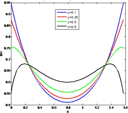
[image:8.595.196.412.513.704.2]

The graphs of the pdf and cdf of the Arc Offset Exponential model are plotted in figure 6 and figure respectively.

(9)

[image:9.595.202.416.83.273.2]

Figure 7. Graph of the cdf of the Arc Offset Exponential distribution

Note: This arc model is symmetric about

4 π

µ =

.

(

)

(

)

(

)

1 2 4 4

2 2 2

4 _{2 cos} _3cos _sin _3cos _sin

g π θ ρ ρ ρ

θ θ θ θ

θ

 

+

 ₊  ₌ ₋ ₋ 

 _{ } _

  _ ₊ ₋ _

 

(

)

(

)

(

)

1 2 4 4 _,

2 2 2

4 _{2 cos} _3cos _sin _3cos _sin

g π θ ρ ρ ρ

θ θ θ θ

θ

 ₊ 

 ₋  ₌ ₋ ₋ 

 _{ } _

  _ ₋ ₊ _

 

4 4

g_π+θ _=g_π −θ _

   .

Hence g is symmetric about

4 π

µ

=

.

The Characteristic Function of the Arc Offset Exponential Model

For p∈ the characteristic function of the Arc Offset Exponential model is

( )

2

( )

0 i p

p

e

g

d

π θ

ϕ

θ

⌠

θ

 ⌡

=

(

)

(

)

(

)

2

2 2 2

0

1 2 2 2 _,

cos sin 2 cos sin cos 2 sin

ip

e d

π

θ ρ ρ ρ _θ

θ θ θ θ θ θ

⌠         ⌡

 ₊ 

 − − 

 

= _ ₊ ₊ ₊ _

where 1 1and 0,

2

π

ρ θ  

− < < _{∈ } _

  (13)

(10)

6. Conclusion

The concept of arc models through offsetting was employed to construct Offset Semicircular Cauchy model. Here we obtained Arc models directly by applying offsetting on a linear bivariate models such as Bivariate Beta and Bivariate Exponential models in which both the variables are defined in [0, 1]and in particular, sum of the variables of Bivariate Beta distribution also lies in [0, 1], irrespective of imposing restriction on circular random variable.

T

hese arc models occurred in natural phenomenon. Some of the newly proposed circular/semicircular/arc models were bimodal models.

In order to fit axial/ l-arc data, the natural choice should be offset circular or semicircular or arc models rather to go in for linear models.

Acknowledgements

Authors would like to thank UGC, New Delhi, India for offering financial assistance to carry out the project under the head of Major Research Project no. F 41-785/2012 (SR) dt. 17-07-2012.

REFERENCES

[1] André L.M. Vilela, F.G.B. Moreira and Adauto J.F. de Souza, Majority –vote model with a bimodal distribution of noises, 2012. http://dx.doi.org/10.1016/j.physa.2012.07.068. [2] Armstrong Nicholas; Kalceff Walter; Cline James;Bonevich

John; Lynch Peter; Tang Chiu; Thompson Steve , X-ray diffraction characterisation of nanoparticles size and shape distributions: application to bimodal distributions, Australian Institute of Physics Publications, Sydney, pp. 1-3. 2004, http://hdl.handle.net/10453/1688

[3] Balakrishnan, N. and Chin Diew Lai, Continuous Bivariate Distributions, Springer. 2008.

[4] Byoung Jin Ahn and Hyoung-Moon Kim. A New Family of Semicircular Models: The Semicircular Laplace Distributions,

Communications of the Korean Statistical Society. Vol.15 (5), 775-781, 2008.

[5] Clinton C Mason, Robert L Hanson, Vicky Ossowski, Li Bian, Leslie J Baier, Jonathan Krakoff and Clifton Bogardus , Bimodal distribution of RNA expression levels in human skeletal muscle tissue, 2011. BMC Genomics, 12:98 doi:10.1186 /1471-2164-12-98.

[6] Dattatreya Rao, A.V, Ramabhadra Sarma, I. and Girija, S.V.S. On Wrapped Version of Some Life Testing Models, Comm Statist, Theor.Meth. 36, 11, pp.2027-2035. 2007.

[7] Dattatreya Rao A.V, Girija S.V.S. and Phani, Y. On Stereographic Logistic Model, Proceedings of NCAMES, AU Engineering College, Visakhapatnam, pp. 139 141. 2011. [8] Fisher, N. I.. Statistical Analysis of Circular Data. Cambridge

University Press, Cambridge. 1993

[9] Girija, S.V.S. Construction of New Circular Models, VDM VERLAG, Germany. ISBN 978-3-639-27939-9. 2010. [10] Girija S.V.S, Radhika A. J. V. and Dattatreya Rao A.V, On

Bimodal Offset Cauchy Distribution, Journal of the Applied Mathematics, Statistics and Informatics (JAMSI), Vol.9, No.1 ,2013.

[11] Jammalamadaka, S.R. and Sen Gupta, A. Topics in Circular Statistics, World Scientific Press, Singapore, (2001).

[12] Mardia, K.V. and Jupp, P.E. Directional Statistics, John Wiley, Chic ester, 2000.

[13] Phani, Y, Girija S.V.S. and Dattatreya Rao A.V, Circular Model Induced by Inverse Stereographic Projection On Extreme-Value Distribution, IRACST –Engineering Science and Technology: An International Journal (ESTIJ), ISSN: 2250-3498,Vol.2, No. 5, pp. 881 888, 2012.

[14] Phani, Y, Girija S.V.S. and Dattatreya Rao A.V, On Construction of Stereographic Semicircular Models, Journal of Applied Probability and Statistics, Vol. 8, No. 1, pp. 75-90, 2013.