DATA PREDICTION FROM A SET OF SAMPLED DATA USING ARTIFICIAL NEURAL NETWORK IN MATLAB SIMULINK

DATA PREDICTION FROM A SET OF SAMPLED DATA USING

ARTIFICIAL NEURAL NETWORK IN MATLAB SIMULINK

1

*Md. Shohel Rana and 2Shakila Zahan

1

Assistant Proessor, Department of Statistics, Islamic University Kushtia-7003, Bangladesh.

2

Department of Statistics Islamic University, Kushtia-7003, Bangladesh.

ABSTRACT

Recent studies have shown the classification and prediction power of

the Neural Networks. It has been demonstrated that a NN can

approximate any continuous function. Neural networks have been

successfully used for forecasting. The classical methods used for time

series prediction like Box-Jenkins or ARIMA assumes that there is a

linear relationship between inputs and outputs. Neural Networks have

the advantage that can approximate nonlinear functions. Classical

statistical and econometric models used to predict efficiently handle

uncertainty nature of data analysis. Prediction of the data from a set of

sampled data is a difficult problem from both theoretical and practical

point of view because the collections of data are influenced by many economic and natural

factors. During the time, many statistical and econometric models have been developed by

researchers for the purpose of prediction of data analysis but this problem remains one of the

major challenges in the field of prediction and forecasting methods. In this paper we

compared the performances of different feed forward and recurrent neural networks and

training algorithms for prediction of the desired data and tried to see the implementation and

comparison of the performance for foreign exchange rate prediction and finally to select the

best method between this two feed forward of that keep the greater influence than the other in

the field of prediction.

KEYWORDS: Artificial Neural Network, MATlab Simulation, Data Prediction.

Volume 7, Issue 18, 333-352. Research Article ISSN 2277– 7105

Article Received on 14 Sept. 2018,

Revised on 05 October 2018, Accepted on 26 October 2018

DOI: 10.20959/wjpr201818-13607

*Corresponding Author

Md. Shohel Rana

Assistant Proessor,

Department of Statistics,

Islamic University

1. INTRODUCTION 1.1 Background

The classical methods used for prediction like Box-Jenkins, ARMA or ARIMA assume that

there is a linear relationship between inputs and outputs. Neural Networks have the advantage

that can approximate any nonlinear functions without any apriority information about the

properties of the data series. Recent studies have shown the classification and prediction

power of the Artificial Neural Networks. It has been demonstrated that a neural network can

approximate any continuous function. Neural networks have been successfully used for

forecasting of data series. This step involves determining the logical consequences of the

hypothesis. One or more predictions are then selected for further testing. The more unlikely

that a prediction would be correct simply by coincidence, then the more convincing it would

be if the prediction were fulfilled; evidence is also stronger if the answer to the prediction is

not already known, due to the effects of hindsight bias. Ideally, the prediction must also

distinguish the hypothesis from likely alternatives; if two hypotheses make the same

prediction, observing the prediction to be correct is not evidence for either one over the other.

These statements about the relative strength of evidence can be mathematically derived

using Bayes' Theorem. Markov Chain is also used to predict different type of prediction

process. In many applications, such as time series analysis, it is possible to estimate the

models that generate the observations. If models can be expressed as transfer functions or in

terms of state-space parameters then smoothed, filtered and predicted data estimates can be

calculated. If the underlying generating models are linear then a minimum-variance Kalman

filter and a minimum-variance smoother may be used to recover data of interest from noisy

measurements. These techniques rely on one-step-ahead predictors which minimize the

variance of the prediction error. When the generating models are nonlinear then stepwise

linearization may be applied within Extended Kalman Filter and smoother recursions.

However, in nonlinear cases, optimum minimum-variance performance guarantees no longer

apply. [An-Sing Chen, Mark T. Leung, Hazem Daouk, Application of neural networks

toforecasting and trading].

1.2 Motivations

This tutorial introduces to the topic of predicting using artificial neural network. In this

particular prediction of data using multi-layer feed-forward neural networks will be

described. Here the well performed programming machine MATlab is used so that we may

of statistical inference. One particular approach to such inference is known as predictive

inference, but the prediction can be undertaken within any of the several approaches to

statistical inference. Indeed, one possible description of statistics is that it provides a means

of transferring knowledge about a sample of a population to the whole population, and to

other related populations, which is not necessarily the same as prediction over time. When

information is transferred across time, often to specific points in time, the process is known

as forecasting. Forecasting usually requires time series methods, while prediction is often

performed on cross-sectional data.

2. Literature review 2.1 Introduction

In science, a prediction is a rigorous, often quantitative, statement, forecasting what would

happen under specific conditions; for example, if an apple fell from a tree it would be

attracted towards the center of the earth by gravity with a specified and constant acceleration.

The scientific method is built on testing statements that are logical consequences of scientific

theories. This is done through repeatable experiments or observational studies. A scientific

theory which is contradicted by observations and evidence will be rejected. New theories that

generate many new predictions can more easily be supported or falsified (see predictive

power). Notions that make no testable predictions are usually considered not to be part of

science (protoscience or nescience) until testable predictions can be made.[S. Haykin, Neural

Networks, Chapter-2, Article- 2.2].

2.2 About Matlab

MATLAB is a programming platform designed specifically for engineers and scientists. The

heart of MATLAB is the MATLAB language, a matrix-based language allowing the most

natural expression of computational mathematics. MATLAB combines a desktop

environment tuned for iterative analysis and design processes with a programming language

that expresses matrix and array mathematics directly that expresses matrix and array

mathematics directly. We can do many things like bellow with MATLAB.

 Analyze data;  Develop algorithms;

 Create models and applications.

The language, apps, and built-in math functions enable you to quickly explore multiple

production by deploying to enterprise applications and embedded devices, as well as

integrating with Simulink and Model-Based Design. A highly efficient language for technical

computation is called MATLAB. It combines visual, computations, and programming in an

easy-to-use environment where problems and solutions are given in well-known

mathematical expressions. It is used for:

 Math and computation;

 Data analysis, exploration, and visualization;  Algorithm development;

 Scientific and engineering graphics;  Modeling, simulation, and prototyping;

 Application development, including Graphical User Interface building.

The data element is considered as an array in a MATLAB interactive system that does not

need dimensioning. It solves many issues regarding technical and computations especially the

ones which include vector and matrix expressions, by using languages like C or FORTRAN

you can write this program in no time. Matrix laboratory is supported by MATLAB and it

was created for giving a user-friendly access to matrix software written by LINPACK and

EISPAKC projects, that together gives the state-of-the-art in matrix computation software.

There has been a periodic evolution of MATLAB over the years with many users providing

input. For basic and advanced mathematics, science, and engineering it is the general

instruction tool used in a university environment. For development, analysis, research, and

higher productivity MATLAB is the apt choice used by the industry. A group of

application-specific solutions namely tool boxes is the main feature of MATLAB. It permits you for

learning and applying specialized technology. There are vast collections of MATLAB

functions in Toolboxes that enhances the ambiance of MATLAB to solve problems of a

particular class. Signal processing, neural networks, wavelets, simulation, fuzzy logic, control

systems and much more are the areas where tool boxes are available.[Introduction to

MATLAB, MATHworks, Chapter-2].

2.3 MATLAB System

It comprises of five main parts 1. Matlab Language

It is an array or matrix language at a higher level with control flow statements, functions,

programming for creating fast and junk throw-away programs, and big programming for

creating difficult and big application programs.

2. Matlab Ambience

It has a set of tools offering lots of provisions that perform with as the MATLAB user or

programmer. It provides help for variable management in your workspace and data transfer.

Developing, managing, debugging, and profiling M-files can be done using the tools of

MATLAB.

3. Graphics Management

Offering higher level commands for two dimensional and three-dimensional data

visualization, animation, image processing, and presentation graphics are included in the

Graphics management. Low-level commands for allowing full customization view of

graphics for building Graphical User Interfaces on your MATLAB applications.

4. Mathematical Library Functions of Matlab

There are various basic operations like sum, cosine, sine, and complex operations collection

of computational algorithms for more sophisticated functions like matrix eigenvalues,

inverse, fast Fourier transforms, and Bessel functions.

5. Matlab Application Program Interface (API)

C and FORTRAN programs for interacting with MATLAB are permitted by the library.

There are other facilities included for calling routines from MATLAB (dynamic linking),

calling MATLAB as a computational engine, MAT-files with reading and writing facility.[S.

Haykin, Neural Networks, Chapter-3, Article- 3.2].

2.4 Model & Simulate Dynamic System Behavior with Matlab, Simulink & Simscape Modeling is a way to create a virtual representation of a real-world system that includes

software and hardware. If the software components of this model are driven by mathematical

relationships, you can simulate this virtual representation under a wide range of conditions to

see how it behaves.

Modeling and simulation are especially valuable for testing conditions that might be difficult

to reproduce with hardware prototypes alone, especially in the early phase of the design

improve the quality of the system design early, thereby reducing the number of errors found

later in the design process.

Common representations for system models include block diagrams, schematics, and state

charts. Using these representations you can model mechatronic systems, control

software, signal processing algorithms, and communications systems. [Introduction to

MATLAB, Mathworks, Chapter- 3].

2.5 Artificial Neural Network in Matlab

The work flow for the general neural network design process has seven primary steps:

 Collect data  Create the network  Configure the network

 Initialize the weights and biases  Train the network

 Validate the network (post-training analysis)  Use the network

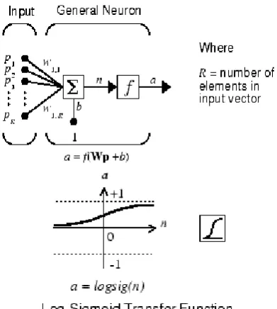
2.5.1 Neuron Model (logsig, tansig, purelin)

An elementary neuron with R inputs is shown below. Each input is weighted with an

appropriate w. The sum of the weighted inputs and the bias forms the input to the transfer

function f. Neurons can use any differentiable transfer function f to generate their output.

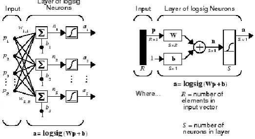
2.5.2 Feed forward Neural Network

A single-layer network of S log sig neurons having R inputs is shown below in full detail on

the left and with a layer diagram on the right.

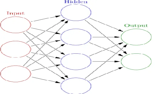
2.5.3 Multilayer Neural Network Architecture

Feed forward networks often have one or more hidden layers of sigmoid neurons followed by

an output layer of linear neurons. Multiple layers of neurons with nonlinear transfer functions

allow the network to learn nonlinear relationships between input and output vectors. The

linear output layer is most often used for function fitting (or nonlinear regression)

problems.[R. Schalkoff, Artificial Neural Networks, Chapter-4].

Figure 2.2: Multilayer Neural Network.

2.6 Prepare Data for Multilayer Neural Networks

Before beginning the network design process, you first collect and prepare sample data. It is

generally difficult to incorporate prior knowledge into a neural network; therefore the

network can only be as accurate as the data that are used to train the network. It is important

that the data cover the range of inputs for which the network will be used.

Multilayer networks can be trained to generalize well within the range of inputs for which

they have been trained. However, they do not have the ability to accurately extrapolate

beyond this range, so it is important that the training data span the full range of the input

space. After the data have been collected, there are two steps that need to be performed

before the data are used to train the network: the data need to be preprocessed, and they need

2.6.1 Choose Neural Network Input-Output Processing Functions

Neural network training can be more efficient if you perform certain preprocessing steps on

the network inputs and targets. This section describes several preprocessing routines that you

can use. (The most common of these are provided automatically when you create a network,

and they become part of the network object, so that whenever the network is used, the data

coming into the network is preprocessed in the same way).

For example, in multilayer networks, sigmoid transfer functions are generally used in the

hidden layers. These functions become essentially saturated when the net input is greater than

three (exp (−3) ≅0.05). If this happens at the beginning of the training process, the gradients

will be very small, and the network training will be very slow. In the first layer of the

network, the net input is a product of the input times the weight plus the bias. If the input is

very large, then the weight must be very small in order to prevent the transfer function from

becoming saturated. It is standard practice to normalize the inputs before applying them to

the network.

2.6.2 Create, Configure & Initialize Multilayer Neural Networks

After the data has been collected, the next step in training a network is to create the network

object. The function feed forward net creates a multilayer feed forward network. If this

function is invoked with no input arguments, then a default network object is created that has

not been configured. The resulting network can then be configured with the configure

command. The configure command configures the network object and also initializes the

weights and biases of the network; therefore the network is ready for training. There are times

when you might want to reinitialize the weights, or to perform a custom initialization.

“Initializing Weights” on page explains the details of the initialization process. You can also

skip the configuration step and go directly to training the network. The train command will

3. METHODOLOGY 3.1 Introduction

Artificial neural networks are relatively crude electronic networks of neurons based on the

neural structure of the brain. They process records one at a time, and learn by comparing their

prediction of the record (largely arbitrary) with the known actual record. The errors from the

initial prediction of the first record is fed back to the network and used to modify the

network's algorithm for the second iteration. These steps are repeated multiple times. Neural

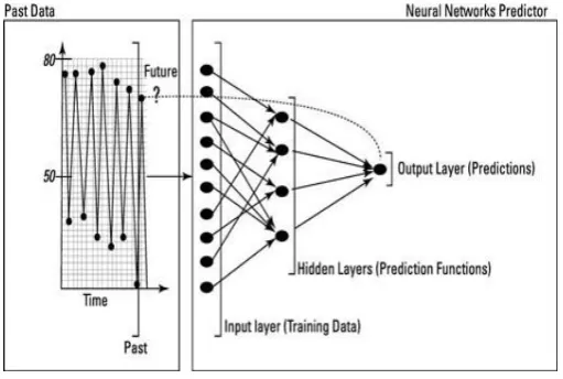
networks can be used to make predictions on time series data such as weather data. A neural

network can be designed to detect pattern in input data and produce an output free of noise.

The structure of a neural-network algorithm has three layers:

 The input layer feeds past data values into the next (hidden) layer. The black circles

represent nodes of the neural network.

 The hidden layer encapsulates several complex functions that create predictors; often

those functions are hidden from the user. A set of nodes (black circles) at the hidden layer

represents mathematical functions that modify the input data; these functions are

called neurons.

 The output layer collects the predictions made in the hidden layer and produces the final

result: the model’s prediction.

Figure 3.1: Layers of a function.

A neuron in an artificial neural network is:

1. A set of input values (xi) with associated weights (wi)

Figure 3.2: Structure of a function.

Neurons are organized into the following layers: input, hidden, and output. The input layer is

composed not of full neurons, but simply of the values in a record that are inputs to the next

layer of neurons. The next layer is the hidden layer of which there could be several. The final

layer is the output layer, where there is one node for each class. A single sweep forward

through the network results in the assignment of a value to each output node. The record is

assigned to the class node with the highest value.[T. Masters, Practical Neural Network

Recipes, Chapter- 4, Article- 4.4].

Figure 3.3: Working process of a neuron.

3.2 Neural Network Models

Neural networks have been achieving great success in natural language processing. Work in

this field with neural networks is mostly based on learning continuous vector representations

of words By representing words in a low dimensional continuous embedding space,

continuous word vectors can encode semantic and syntactic features of words and are

supposed to be superior to conventional methods that treat words as discrete symbols or use

Our neural network based approaches to sequence prediction are developed on top of the

continuous word vectors that are trained using Continuous Bag-of-Words Model (CBOW)

proposed and implemented by. With pre trained word vectors, we transform the original

discrete symbol sequences as follows. Given a sequence of length L, we first right pad it with

the symbol END, which indicates the end of the sequence. Assume that we predict the next

symbol from the previous k symbols; we also need to left pad the sequence with k DUMMY

symbols, so that we can construct the inputs to the classifier when predicting the first k

symbols of the sequence. We then construct the training set for the neural network classifier:

for each symbol s in the sequence (other than the DUMMY symbols), we sequentially

concatenate the word vectors of its previous k symbols as the input and regard s as the label.

Figure in below gives an example of this procedure.

Figure 3.4: Sequence layers of Neural Network.

We use three different neural network classifiers as described below.

 MLP is a feed forward artificial neural network model that consists of multiple layers of

nodes in a directed graph, with each layer fully connected to the next one. Each node in

intermediate layers (hidden layers) is a neuron with a nonlinear activation function (tanh,

ReLU, or sigmoid). The output layer is a soft max layer that implements soft max

function for classification and cross-entropy cost function is used while training the MLP

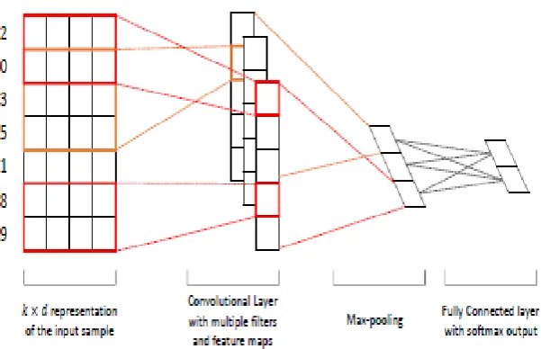
 CNN is a feed forward neural network that contains convolution layers with a nonlinear

activation function such as ReLU. Besides, CNN could also contain pooling layers that

are usually used immediately after each convolution layer. In SPiCe we employ the CNN

model. For simplicity, the input layer only contains a static channel, and we do not

enforce the L2-norm constraint on the weight vectors that parameterize the soft max

function, which Zhang and Wallace (2015) found generally did not improve performance

much. Figure 2 shows our CNN model architecture for sequence prediction.

 LSTM is a special kind of recurrent neural network (RNN) architecture that was proposed

by Hoch Reiter and Schmidhuber (1997) to combat the vanishing gradient problem.

Featured with the gating mechanism, LSTM is well-suited to model long term

dependencies and has been successfully applied to language modeling. In P Spice we use

the standard LSTM architecture, and the hidden state of the LSTM model is fed to the

logistic regression classifier.

3.3 Feed Forward

The feed forward, back-propagation architecture was developed in the early 1970s by several

independent sources (Werbor, Parker, Rumelhart, Hinton, and Williams). This independent

co-development was the result of a proliferation of articles and talks at various conferences

that stimulated the entire industry. Currently, this synergistically developed back-propagation

architecture is the most popular and effective model for complex, multi-layered networks. Its

greatest strength is in non-linear solutions to ill-defined problems. The typical

back-propagation network has an input layer, an output layer, and at least one hidden layer.

Theoretically, there is no limit on the number of hidden layers, but typically there are just one

or two. Some studies have shown that the total number of layers needed to solve problems of

any complexity is five (one input layer, three hidden layers, and an output layer). Each layer

is fully connected to the succeeding layer.

The training process normally uses some variant of the Delta Rule, which starts with the

calculated difference between the actual outputs and the desired outputs. Using this error,

connection weights are increased in proportion to the error times, which are a scaling factor

for global accuracy. This means that the inputs, the output, and the desired output all must be

present at the same processing element. The most complex part of this algorithm is

determining which input contributed the most to an incorrect output and how to modify the

no need to change its weights.) To solve this problem, training inputs are applied to the input

layer of the network, and desired outputs are compared at the output layer. During the

learning process, a forward sweep is made through the network, and the output of each

element is computed layer by layer. The difference between the output of the final layer and

the desired output is back-propagated to the previous layer(s), usually modified by the

derivative of the transfer function. The connection weights are normally adjusted using the

Delta Rule. This process proceeds for the previous layer(s) until the input layer is reached.

3.4 Structuring the Network

The number of layers and the number of processing elements per layer are important

decisions. To a feed forward, these parameters back-propagation topology, are also the most

ethereal - they are the art of the network designer. There is no quantifiable, best answer to the

layout of the network for any particular application. There are only three general rules picked

up over time and followed by most researchers and engineers applying this architecture to

their problems.

Rule One: As the complexity in the relationship between the input data and the desired output increases, the number of the processing elements in the hidden layer should also

increase.

Rule Two: If the process being modeled is separable into multiple stages, then additional hidden layer(s) may be required. If the process is not separable into stages, then additional

layers may simply enable memorization of the Training Set, and not a true general solution.

Rule Three: The amount of training data available sets an upper bound for the number of processing elements in the hidden layer(s). To calculate this upper bound, use the number of

cases in the Training Set and divide that number by the sum of the number of nodes in the

input and output layers in the network. Then divide that result again by a scaling factor

between five and ten. Larger scaling factors are used for relatively less noisy data. If too

many artificial neurons are used, the Training Set will be memorized, not generalized, and the

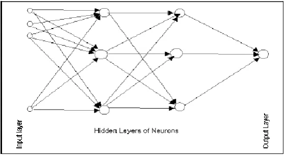
Figure 3.5: Structure of ANN.

4. RESULT AND ANALYSIS 4.1 Introduction

Predicting is making claims about something that will happen, often based on information

from past and from current state. Everyone solves the problem of prediction every day with

various degrees of success. For example weather, harvest, energy consumption, movements

of foreign exchange currency pairs or of shares of stocks, earthquakes, and a lot of other stuff

needs to be predicted. In technical domain predictable parameters of a system can be often

expressed and evaluated using equations - prediction is then simply evaluation or solution of

such equations. However, practically we face problems where such a description would be

too complicated or not possible at all. In addition, the solution by this method could be very

complicated computationally, and sometimes we would get the solution after the event to be

predicted happened.

For the computation of this study first the topic of prediction will be described together with

classification of prediction into types. After that, the prediction using neural networks (NNs)

will be described. The focus will be on the creation of a training set from collected data. For

the illustration of this topic MATlab from MATH works are available that illustrate the

creation of a training set and that show the result of a prediction using a neural network of

both on primary and secondary data.

4.2 Prediction

Neural networks can be used for prediction with various levels of success. The advantage of

then includes automatic learning of dependencies only from measured data without any need

network is trained from the historical data with the hope that it will discover hidden

dependencies and that it will be able to use them for predicting into future. In other words,

neural network is not represented by an explicitly given model. It is more a black box that is

able to learn something.

It is possible to predict various types of data, however in the rest of this text we will focus on

predicting of time series. Time series shows the development of a value in time. Of course,

the value can be influenced by also other factors than just time. Time series represents

discrete history of a value and from a continuous function it can be obtained using sampling.

The prediction type can be classified according to various criteria. Basic criteria are,

 Data that we have for teaching prediction and for prediction.

 What we want to predict - value or trend.

4.3 Predicting Value or Trend

When we want to get exact value (or more values) of a variable in future, then we are

predicting value. Other possibility is to predict trend of a variable, i.e., whether the value will

go up or down without considering size of the change - then we are predicting trend. When

predicting trend we are in fact classifying into two (or three) classes - up and down (or no

significant change). Prediction of a close value is generally easier than predicting a trend.

Besides trend we may also want to predict other parts of the trend, such as moving average

change etc.

4.4 Data for Prediction

For time series predicting we usually have values of a variable in equidistant intervals - then

we can try to predict the development of the value based on historical values and time only.

In this case the historical time series should be long enough and dense enough.

We can have additional information to time series, such as derivation. This information can

be then used for more exact prediction. Important information can be added using so

called interventional variables (intervention indicators), which represent information about

time series or information about the period into which we predict. For example when

predicting energy consumption then knowing whether we predict for Monday or Saturday can

improve the prediction dramatically - this information does not follow from time series

explicitly and must be added. It is usually very helpful to use the values of intervention

We can also have information about other related variables, preferably also in time series.

From the history of related variables we can reason about other variables. The relation can be

expressed in various ways. An example is a static (or slowly changing) sum of two variables.

It does not have to be expressed explicitly - for example changes of prices of stocks of shares

in one sector are dependent, but can be hard to express in a computational way. This kind of

information is selected in a hope that it will cohere with the predicted value, but we do not

have to be sure about it. The field of data mining can help with selecting appropriate

information and its interpretation.

4.5 Prediction using ANN

The advantage of the usage of neural networks for prediction is that they are able to learn

from examples only and that after their learning is finished, they are able to catch hidden and

strongly non-linear dependencies, even when there is a significant noise in the training set.

The disadvantage is that NNs can learn the dependency valid in a certain period only. The

error of prediction cannot be generally estimated.

4.6 Graphical Output Analysis

The above figure shows the structure of Artificial Neural Network in Matlab where the four

types of layers are displayed- Input Layer, Hidden Layer, Output Layer and final the Output.

The working process of a neural network happens in the hidden layer. In this layer there are

different types of probabilities results but the most probable out is displayed in the output

This figure shows the graphical representation of the most probable output of the following

project. Here the main line shows the standard data and the round shapes circles shows the

probable outputs.

This graphical presentation shows the different states of the training. The gradient, the

This graph shows the comparison between the main standard expected outputs with the given

input. Here a little bit of fluctuation is occurred due to training period. The blue line shows

the train state and the green and the red line shows the validation and test state. The white

line notifies the most expected output state.

4.7 Predicted Data

0.32976 0.38914 0.93677 0.44013

Accurate prediction and forecasting are very difficult in some areas, such as natural

disasters, pandemics, demography, dynamics and meteorology. For example, it is possible to

predict the occurrence of solar cycles, but their exact timing and magnitude is much more

difficult. Established science makes useful predictions which are often extremely reliable and

accurate; for example, eclipses are routinely predicted.

New theories make predictions which allow them to be disproved by reality. For example,

predicting the structure of crystals at the atomic level is a current research challenge. In the

early 20th century the scientific consensus was that there existed an absolute frame of

reference, which was given the name aluminiferous ether. The existence of this absolute

frame was deemed necessary for consistency with the established idea that the speed of light

is constant. The famous Michelson-Morley experiment demonstrated that predictions

deduced from this concept were not borne out in reality, thus disproving the theory of a n

explanation for the seeming inconsistency between the constancy of the speed of light and the

non-existence of a special, preferred or absolute frame of reference.

5. SUMMARY AND CONCLUSION

Neural networks are suitable for predicting because of learning only from examples, without

any need to add additional information that can bring more confusion than prediction effect.

Neural networks are able to generalize and are resistant to noise. On the other hand, it is

generally not possible to determine exactly what a neural network learned and it is also hard

to estimate possible prediction error. However, neural networks were often successfully used

for predicting data. They are ideal especially when we do not have any other description of

the observed series.

REFERENCES

1. S. Haykin, Neural Networks, New York, NY: Nacmillan College Publishing Company,

Inc., 1994.

2. H. Abdi, D. Valentin, B. Edelman, Neural Networks, Thousand Oaks, CA: SAGE

Publication Inc., 1999.

3. T. Masters, Practial Neural Network Recipes in C, Toronto, ON: Academic Press, Inc.,

1993.

4. R. Schalkoff, Artificial Neural Networks, Toronto, ON: the McGraw-Hill Companies,

Inc., 1997.

5. S. M. Weiss and C. A. Kulikowski, Computer Systems That Learn, San Mateo, CA:

Morgan Kaufmann Publishers, Inc., 1991.

6. P. D. Wasserman, Neural Computing: Theory and Practice, New York, NY: Van

Nostrand Reinhold, 1989.

7. Ye Zhang and Byron Wallace. A sensitivity analysis of and practitioners' guide to

convolutional neural networks for sentence classification.

8. An-Sing Chen, Mark T. Leung, HazemDaouk, Application of neural networks to an

emerging financial market: forecasting and trading the Taiwan Stock Index, Computers &

Operations Research, 2003; 30: 901–923.

9. Man-Chung Chang, Chi-Cheong Wong, Chi-Chung Lam, Financial Time Series

Forecasting by Neural Network Using Conjugate Gradient Learning Algorithm and

Multiple Linear Regression Weight Initialization, Computing in Economics and Finance

10.Lee A. Feldkamp, Danil V. Prokhorov, Charles F. Eagen and Fumin Yuan, Enhaced

multi-stream Kalman filter training for recurrent networks, in J. Suykens and J.

Vandewalle (Eds.) Nonlinear Modeling: Advanced Black-Box Techniques, pp. 29-53,

Kluwer Academic Publishers, 1998.

11.Igel, C., Hüsken, M., 2000. Improving the Rprop Learning Algorithm, Proceedings of the

Second International Symposium on Neural Computation, pp. 115–121, ICSC Academic

Press.

12.Herbert Jaeger, Tutorial on training recurrent neural networks, covering BPTT, RTRL,

EKF and the "echo state network" approach, Technical Report GMD Report 159, German

National Research Center for Information Technology, 2002.

13.V. Kondratenko, Yu. A Kuperin, Using Recurrent Neural Networks To Forecasting of

Forex, Condensed Matter, Statistical Finance, 2003.

14.Mehdi Khashei, Mehdi Bijari, Gholam Ali Raissi Ardali, Hybridization of autoregressive

integrated moving average (ARIMA) with probabilistic neural networks (PNNs),

Computers & Industrial Engineering, 2012; 63: 37–45.

15.Adewole Adetunji Philip, Akinwale Adio Taofiki, Akintomide Ayo Bidemi, Artificial

Neural Network Model for Forecasting Foreign Exchange Rate, World of Computer

Science and Information Technology Journal (WCSIT), 2011; 1(3): 110-118.

16.Tommaso Proietti, Helmut Lütkepohl, “Does the Box–Cox transformation help in

forecasting macroeconomic time series?, International”, Journal of Forecasting, 2013; 29:

88–99.

17.R. Rojas, Neural Networks, Springer-Verlag, Berlin, 1996.

18.Hong Tan, Neural Network for Stock Forecasting, Master of Science in Electrical