Real-time Systems
Specification, Verification and
Analysis
Edited by Mathai Joseph
Tata Research Development & Design Centre
Revised version with corrections
under
ISBN 0-13-455297-0
This version incorporates corrections to and changes from the original
edition.
This version is made
available for research,
teaching and personal use
only.
Copies may be made for
non-commercial use only.
Enquiries for other uses to
the Editor
Contents
Preface vii
Contributors xii
1 Time and Real-time 1
Mathai Joseph
Introduction 1 1.1 Real-time computing 2 1.2 Requirements, specification and implementation 3 1.3 The mine pump 5 1.4 How to read the book 11 1.5 Historical background 12 1.6 Exercises 14
2 Fixed Priority Scheduling – A Simple Model 15
Mathai Joseph
Introduction 15 2.1 Computational model 16 2.2 Static scheduling 18 2.3 Scheduling with priorities 19 2.4 Simple methods of analysis 20 2.5 Exact analysis 24 2.6 Extending the analysis 29 2.7 Historical background 30 2.8 Exercises 31
3 Advanced Fixed Priority Scheduling 32
Alan Burns and Andy Wellings
Introduction 32 3.1 Computational model 32 3.2 Advanced scheduling analysis 38 3.3 Introduction to Ada 95 50 3.4 The mine pump 53 3.5 Historical background 64 3.6 Further work 64 3.7 Exercises 65
4 Dynamic Priority Scheduling 66
Krithi Ramamritham
Introduction 66 4.1 Programming dynamic real-time systems 69 4.2 Issues in dynamic scheduling 75 4.3 Dynamic priority assignment 76 4.4 Dynamic best-effort approaches 80 4.5 Dynamic planning-based approaches 83 4.6 Practical considerations in dynamic scheduling 90 4.7 Historical background 93 4.8 Further work 94 4.9 Exercises 95
5 Assertional Specification and Verification 97
Jozef Hooman
6 Specification and Verification in Timed CSP 147
Steve Schneider
Introduction 147 6.1 The language of real-time CSP 147 6.2 Observations and processes 156 6.3 Specification 162 6.4 Verification 164 6.5 Case study: the mine pump 169 6.6 Historical background 178 6.7 Exercises 180
7 Specification and Verification in DC 182
Zhiming Liu
Introduction 182 7.1 Modelling real-time systems 182 7.2 Requirements 184 7.3 Assumptions 188 7.4 Design 189 7.5 The basic duration calculus (DC) 191 7.6 The mine pump 198 7.7 Specification of scheduling policies 202 7.8 Probabilistic duration calculus (PDC) 205 7.9 Historical background 224 7.10 Further work 225 7.11 Exercises 227
8 Real-time Systems and Fault-tolerance 229
Henk Schepers
Introduction 229 8.1 Assertions and correctness formulae 230 8.2 Formalizing a failure hypothesis 232 8.3 A proof rule for failure prone processes 234 8.4 Reliability of the mine pump 236 8.5 Soundness and completeness of the new proof rule 250 8.6 Historical background 254 8.7 Exercises 256
References 259
Preface
The field of real-time systems has not traditionally been hospitable to newcomers: on the one hand there are experts who seem to rely on experience and a few specialized docu-ments and, on the other, there is a vast and growing catalogue of technical papers. There are very few textbooks and the most successful publications are probably collections of past papers carefully selected to cover different views of the field. As interest has grown, so has the community, and the more recent papers are spread over a large range of pub-lications. This makes it particularly difficult to keep in touch with all the new develop-ments.
If this is distressing to the newcomer, it is of no less concern to anyone who has to teach a course on real-time systems: one has only to move a little beyond purely technical concerns to notice how quickly the teachable material seems to disappear in a cloud of opinions and a range of possibilities. It is not that the field lacks intellectual challenges or that there is not enough for a student to learn. On the contrary, the problem seems to be a question of where to start, how to relate practical techniques with methods of analysis, analytical results with theories and, more crucially, how to decide on the objectives of a course.
This book provides a detailed account of three major aspects of real-time systems: program structures for real-time, timing analysis using scheduling theory and specifica-tion and verificaspecifica-tion in different frameworks. Each chapter focuses on a particular tech-nique: taken together, they give a fairly comprehensive account of the formal study of real-time systems and demonstrate the effectiveness and applicability of mathematically based methods for real-time system design. The book should be of interest to computer scientists, engineers and practical system designers as it demonstrates also how these new methods can be used to solve real problems.
Chapters have different authors and each focuses on a particular topic, but the material has been written and edited so that the reader should notice no abrupt changes when mov-ing from one chapter to another. Chapters are linked with cross-references and through their description and analysis of a common example: the mine pump (Burns & Lister, 1991; Mahony & Hayes, 1992). This allows the reader to compare the advantages and
limitations of different techniques. There are a number of small examples in the text to illustrate the theory and each chapter ends with a set of exercises.
The idea for the book came originally from material used for the M.Sc. module on real-time systems at the University of Warwick. This module has now been taught by several of the authors over the last three years and has been attended by both students and visiting participants. However, it was planned that the book would contain a more comprehensive treatment of the material than might be used in a single course. This al-lows teachers to draw selectively on the material, leaving some parts out and others as further reading for students. Some possible course selections are outlined in Chapter 1 but many more are possible and the choice will be governed by the nature of the course and the interests and preparation of the students. Part of the material has been taught by the authors in advanced undergraduate courses in computer science, computer engineer-ing and related disciplines; selections have also been used in several different postgrad-uate courses and in short courses for industrial groups. So the material has been used successfully for many different audiences.
The book draws heavily on recent research and can also serve as a source book for those doing research and for professionals in industry who wish to use these techniques in their work. The authors have many years of research experience in the areas of their chapters and the book contains material with a maturity and depth that would be difficult for a single author to achieve, certainly on a short time-scale.
Acknowledgements
Each chapter has been reviewed by another author and then checked and re-drafted by the editor to make the style of presentation uniform. This procedure has required a great deal of cooperation and understanding from the authors, for which the editor is most grateful. Despite careful scrutiny, there will certainly be inexcusable errors lurking in corners and we would be very glad to be informed of any that are discovered.
We are very grateful to the reviewers for comments on the draft and for providing us with the initial responses to the book. Anders Ravn read critically through the whole manuscript and sent many useful and acute observations and corrections. Matthew Wa-hab pointed out a number of inconsistencies and suggested several improvements. We are also glad to acknowledge the cooperation of earlier ‘mine pump’ authors, Andrew Lister, Brendan Mahony and Ian Hayes.
In addition, particular thanks are due to many other people for their comments on dif-ferent chapters.
Chapters 1, 2: Tomasz Janowski made several useful comments, as did students of
the M.Sc. module on real-time systems and the Warwick undergraduate course,
Verifica-tion and ValidaVerifica-tion. Steve Schneider’s specificaVerifica-tion in Z of the mine pump was a useful
template during the development of the specification in Chapter 1.
Chapter 4: Gerhard Fohler, Swamy Kutti and Arcot Sowmya commented on an earlier
draft. Thanks are also due to the present and past members of the real-time group at the University of Massachusetts.
for improvement.
Chapter 6: Jim Davies, Bruno Dutertre, Gavin Lowe, Paul Mukherjee, Justin Pearson,
Ken Wood and members of the ESPRIT Basic Research Action CONCUR2 provided comments at various stages of the work.
Chapter 7: Zhou Chaochen was a source of encouragement and advice during the
writ-ing of this chapter.
The book was produced using LATEX2e, aided by the considerable ingenuity, skill and
perseverance of Steven Haeck, with critical tips from Jim Davies and with help at many stages from Jeff Smith.
Finally, the book owes a great deal to Jackie Harbor of Prentice Hall International, who piloted the project through from its start, and to Alison Stanford, who was Senior Pro-duction Editor. Their combined efforts made it possible for the writing, editing and re-viewing of the book to be interleaved with its production so that the whole process could be completed in 10 months.
The Series editor, Tony Hoare, encouraged us to start the book and persuaded us not to be daunted by the task of editing it into a cohesive text. All of us, editor and authors, owe a great deal for this support.
Preface to Revised Edition
In the five years that have passed since the original edition of the book was published, the field of real-time systems has grown at a breathtaking rate. Most notably, embedded systems have become a separate field of study from other real-time control systems and applications of
embedded systems have spread from the original domain of machinery and transportation to hand-held devices, like organizers, personal digital assistants and mobile telephones. Along with this, the nature of the problems to be faced has also changed. Reliability, usability and adaptability are now added to the factors that must be studied and analyzed when designing a real-time embedded system. And with widespread personal use taking place, it is not just usability but also reliability under unspecified use (e.g. incorrect operation, environmental change, component and subsystem failure) that must be demonstrated.
Nevertheless, the basic principles for the analysis, specification and verification of real-time systems remain unchanged. Whether using a design method such as real-time UML, or more traditional software engineering methods, timing properties must still be determined in conjunction with functional properties. New methods may further systematize the ways in which real-time systems are designed but timing analysis will still need to be done using methods such as those illustrated in this book.
This book has been in use for teaching several courses on real-time systems. With requests for copies still coming from different parts of the world, for both teaching and personal use, the contributors quickly decided that there would be a continued readership for some time to come. The only choice was between producing a revised and corrected edition and collaborating once again to produce a wholly new book. While the second choice would be closer to ideal, the other commitments of the authors have led us to choose the first alternative as being both practical and capable of early completion. Many of the contributors have changed their earlier affiliations and locations and some even their roles, making collaboration at the same level difficult to contemplate. We therefore leave the task of producing a new text on the specification, verification and analysis of real-time systems to other authors, wishing them well and assuring them of our support and of our belief that such as task is well worth doing.
The original edition of this book was published by Prentice-Hall International, London, in 1996. A revised edition with corrections and some changes was planned but, as the title was discontinued by the publishers in 1998, never saw light of day. This revised edition incorporating the corrections and changes is now being made available free of cost for research, teaching and personal use.
Tata Research Development & Design Centre 54B Hadapsar Industrial Estate
Pune 411 013, India
x
Contributors
Professor Alan Burns [email protected]
Department of Computer Science University of York,
Heslington
York YO10 5DD, UK
Dr. Jozef Hooman [email protected]
Computing Science Institute University of Nijmegen P.O. Box 9010
6500 GL Nijmegen, The Netherlands
Professor Mathai Joseph [email protected]
Tata Research Development & Design Centre 54B Hadapsar Industrial Estate
Pune 411 013, India
Dr. Zhiming Liu [email protected]
Department of Mathematics and Computer Science University of Leicester
Leicester LE1 7RH, UK
Professor Krithi Ramamritham [email protected]
Department of Computer Science and Engineering Indian Institute of Technology
Powai
Mumbai 400 076, India
Dr. Ir. Henk Schepers [email protected]
Philips Research Laboratories Information & Software Technology Prof. Holstlaan 4
5656 AA Eindhoven, The Netherlands
Dr. Steve Schneider [email protected]
Department of Computer Science Royal Holloway, University of London Egham, Surrey TW20 0EX, UK
Professor A.J. Wellings [email protected]
Department of Computer Science University of York
Heslington
York YO10 5DD, UK
Time and Real-time
Mathai Joseph
Introduction
There are many ways in which we alter the disposition of the physical world. There are obvious ways, such as when a car moves people from one place to another. There are less obvious ways, such as a pipeline carrying oil from a well to a refinery. In each case, the purpose of the ‘system’ is to have a physical effect within a chosen time-frame. But we do not talk about a car as being a real-time system because a moving car is a closed
system consisting of the car, the driver and the other passengers, and it is controlled from
within by the driver (and, of course, by the laws of physics).
Now consider how an external observer would record the movement of a car using a pair of binoculars and a stopwatch. With a fast moving car, the observer must move the binoculars at sufficient speed to keep the car within sight. If the binoculars are moved too fast, the observer will view an area before the car has reached there; too slow, and the car will be out of sight because it is ahead of the viewed area. If the car changes speed or direction, the observer must adjust the movement of the binoculars to keep the car in view; if the car disappears behind a hill, the observer must use the car’s recorded time and speed to predict when and where it will re-emerge.
Suppose the observer replaces the binoculars by an electronic camera which requires
n seconds to process each frame and determine the position of the car. As when the car is
behind a hill, the observer must predict the position of the car and point the camera so that it keeps the car in the frame even though it is ‘seen’ only at intervals of n seconds. To do this, the observer must model the movement of the car and, based on its past behaviour, predict its future movement. The observer may not have an explicit ‘model’ of the car and may not even be conscious of doing the modelling; nevertheless, the accuracy of the prediction will depend on how faithfully the observer models the actual movement of the car.
Finally, assume that the car has no driver and is controlled by commands radioed by the observer. Being a physical system, the car will have some inertia and a reaction time, and the observer must use an even more precise model if the car is to be controlled
fully. Using information obtained every n seconds, the observer must send commands to adjust throttle settings and brake positions, and initiate changes of gear when needed. The difference between a driver in the car and the external observer, or remote controller, is that the driver has a continuous view of the terrain in front of the car and can adjust the controls continuously during its movement. The remote controller gets snapshots of the car every n seconds and must use these to plan changes of control.
1.1
Real-time computing
A real-time computer controlling a physical device or process has functions very similar to those of the observer controlling the car. Typically, sensors will provide readings at periodic intervals and the computer must respond by sending signals to actuators. There may be unexpected or irregular events and these must also receive a response. In all cases, there will be a time-bound within which the response should be delivered. The ability of the computer to meet these demands depends on its capacity to perform the necessary computations in the given time. If a number of events occur close together, the computer will need to schedule the computations so that each response is provided within the required time-bounds. It may be that, even so, the system is unable to meet all the possible unexpected demands and in this case we say that the system lacks sufficient resources (since a system with unlimited resources and capable of processing at infinite speed could satisfy any such timing constraint). Failure to meet the timing constraint for a response can have different consequences: in some cases, there may be no effect at all; in other cases, the effects may be minor and correctable; in yet other cases, the results may be catastrophic.
Looking at the behaviour required of the observer allows us to define some of the prop-erties needed for successful real-time control. A real-time program must
interact with an environment which has time-varying properties, exhibit predictable time-dependent behaviour, and
execute on a system with limited resources.
system to manifest predictable time-dependent behaviour it is thus necessary for the en-vironment to make predictable demands.
With a human observer, the ability to react in time can be the result of skill, training, experience or just luck. How do we assess the real-time demands placed on a computer system and determine whether they will be met? If there is just one task and a single processor computer, calculating the real-time processing load may not be very difficult. As the number of tasks increases, it becomes more difficult to make precise predictions; if there is more than one processor, it is once again more difficult to obtain a definite prediction.
There may be a number of factors that make it difficult to predict the timing of re-sponses.
A task may take different times under different conditions. For example, predicting
the speed of a vehicle when it is moving on level ground can be expected to take less time than if the terrain has a rough and irregular surface. If the system has many such tasks, the total load on the system at any time can be very difficult to calculate accurately.
Tasks may have dependencies: Task A may need information from Task B before
it can complete its calculation, and the time for completion of Task B may itself be variable. Under these conditions, it is only possible to set minimum and maximum bounds within which Task A will finish.
With large and variable processing loads, it may be necessary to have more than
one processor in the system. If tasks have dependencies, calculating task comple-tion times on a multi-processor system is inherently more difficult than on a single-processor system.
The nature of the application may require distributed computing, with nodes
con-nected by communication lines. The problem of finding completion times is then even more difficult, as communication between tasks can now take varying times.
1.2
Requirements, specification and implementation
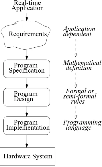
The demands placed on a real-time system arise from the needs of the application and are often called the requirements. Deciding on the precise requirements is a skilled task and can be carried out only with very good knowledge and experience of the application. Failures of large systems are often due to errors in defining the requirements. For a safety-related real-time system, the operational requirements must then go through a hazard and risk analysis to determine the safety requirements.
Requirements ApplicationReal-time
Program Specification
Program Design
Program Implementation
Hardware System
Application
Mathematical dependent
definition
Formal or
rules semi-formal
[image:16.595.232.410.81.372.2]language Programming
Figure 1.1 Requirements, specification and implementation
A specification is a mathematical statement of the properties to be exhibited by a sys-tem. A specification should be abstract so that
it can be checked for conformity against the requirement, and
its properties can be examined independently of the way in which it will be
imple-mented, i.e. as a program executing on a particular system.
This means that a specification should not enforce any decisions about the structure of the software, the programming language to be used or the kind of system on which the pro-gram is to be executed: these are properly implementation decisions. A specification is transformed into an application by taking design decisions, using formal or semi-formal rules, and converted into a program in some language (see Figure 1.1).
0 0 0 0 0 0 1 1 1 1 1 1 0 0 0 0 0 1 1 1 1 1 0 0 0 1 1 1 0 0 0 0 0 0 0 0 0 0 0 1 1 1 1 1 1 1 1 1 1 1 A B C E D Pump Controller Pump Sump Log Operator
High water sensor Airflow sensor Methane sensor
Low water sensor
Carbon Monoxide sensor A
[image:17.595.198.509.82.342.2]B C D E
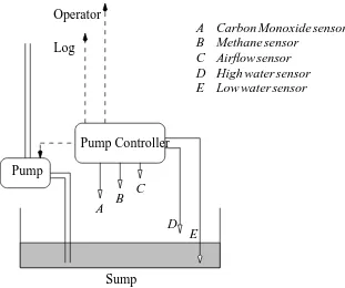
Figure 1.2 Mine pump and control system (adapted from Burns and Lister, 1991)
1.3
The mine pump
Water percolating into a mine is collected in a sump to be pumped out of the mine (see Figure 1.2). The water level sensors D and E detect when water is above a high and a low level respectively. A pump controller switches the pump on when the water reaches the high water level and off when it goes below the low water level. If, due to a failure of the pump, the water cannot be pumped out, the mine must be evacuated within one hour.
The mine has other sensors (A, B, C) to monitor the carbon monoxide, methane and airflow levels. An alarm must be raised and the operator informed within one second of any of these levels becoming critical so that the mine can be evacuated within one hour. To avoid the risk of explosion, the pump must be operated only when the methane level is below a critical level.
Human operators can also control the operation of the pump, but within limits. An operator can switch the pump on or off if the water is between the low and high water levels. A special operator, the supervisor, can switch the pump on or off without this restriction. In all cases, the methane level must be below its critical level if the pump is to be operated.
Safety requirements
From the informal description of the mine pump and its operations we obtain the follow-ing safety requirements:
1. The pump must not be operated if the methane level is critical. 2. The mine must be evacuated within one hour of the pump failing.
3. Alarms must be raised if the methane level, the carbon monoxide level or the air-flow level is critical.
Operational requirement
The mine is normally operated for three shifts a day, and the objective is for no more than one shift in 1000 to be lost due to high water levels.
Problem
Write and verify a specification for the mine pump controller under which it can be shown that the mine is operated whenever possible without violating the safety requirements.
Comments
The specification is to be the conjunction of two conditions: the mine must be operated when possible, and the safety requirements must not be violated. If the specification read ‘The mine must not be operated when the safety requirements are violated’, then it could be trivially satisfied by not operating the mine at all! The specification must obviate this easy solution by requiring the mine to be operated when it is safely possible.
Note that the situation may not always be clearly defined and there may be times when it is difficult to determine whether operating the mine would violate the safety require-ments. For example, the pump may fail when the water is at any level; does the time of one hour for the evacuation of the mine apply to all possible water levels? More cru-cially, how is pump failure detected? Is pump failure always complete or can a pump fail partially and be able to displace only part of its normal output?
It is also important to consider under what conditions such a specification will be valid. If the methane or carbon monoxide levels can rise at an arbitrarily fast rate, there may not be time to evacuate the mine, or to switch off the pump. Unless there are bounds on the rate of change of different conditions, it will not be possible for the mine to be operated and meet the safety requirements. Sensors operate by sampling at periodic intervals and the pump will take some time to start and to stop. So the rate of change of a level must be small enough for conditions not to become dangerous during the reaction time of the equipment.
The control system obtains information about the level of water from the Highwater and Lowwater sensors and of methane from the Methane sensor. Detailed data is needed about the rate at which water can enter the mine, and the frequency and duration of met-hane leaks; the correctness of the control software is predicated on the accuracy of this information. Can it also be assumed that the sensors always work correctly?
evac-uation. For example, can a mine be evacuated more than once in a shift or, following an evacuation, is the shift considered to be lost? If the mine is evacuated, it would be normal for a safety procedure to come into effect and for automatic and manual clearance to be needed before operation of the mine can resume. This information will make it possible to decide on how and when an alarm is reset once it has been raised.
1.3.1 Developing a specification
The first task in developing a specification is to make the informal description more pcise. Some requirements may be very well defined but it is quite common for many re-quirements to be stated incompletely or with inconsistencies between rere-quirements. For example, we have seen that there may be conditions under which it is not possible to meet both the safety requirements and the operational requirement; unfortunately, the descrip-tion gives us no guidance about what should be done in this case. In practice, it is then necessary to go back to the user or the application engineer to ask for a more precise def-inition of the needs and to resolve inconsistencies. The process of converting informally stated requirements into a more precise form helps to uncover inconsistencies and inad-equacies in the description, and developing a specification often needs many iterations.
We shall start by trying to describe the requirements in terms of some properties, using a simple mathematical notation. This is a first step towards making a formal specification and we shall see various different, more complete, specifications of the problem in later chapters.
Properties will be defined with simple predicate calculus expressions using the logical operators^ (and),_ (or),) (implies) and, (iff), and the universal quantifier8 (for
all). The usual mathematical relational operators will be used and functions, constants
and variables will be typed. We use
F : T1!T2
for a function F from type T1 (the domain of the function) to type T2 (the range of the
function) and a variable V of type T will be defined as V : T. An interval from C1 to
C2will be represented as[C1;C2]if the interval is closed and includes both C1and C2,
as(C1;C2]if the interval is half-open and includes C2and not C1 and as[C1;C2)if the
interval is half-open and includes C1and not C2.
Assume that time is measured in seconds and recorded as a value in the set Time and the depth of the water is measured in metres and is a value in the set Depth; Time and
Depth are the set of real numbers.
S1: Water level
The depth of the water in the sump depends on the rate at which water enters and leaves the sump and this will change over time. Let us define the water level Water at any time to be a function from Time to Depth:
Let Flow be the rate of change of the depth of water measured in metres per second and be represented by the real numbers; WaterIn and WaterOut are the rates at which water enters and leaves the sump and, since these rates can change, they are functions from
Time to Flow:
WaterIn;WaterOut : Time!Flow
The depth of water in the sump at time t2 is the sum of the depth of water at an earlier time t1and the difference between the amount of water that flows in and out in the time
interval[t 1;t
2]. Thus8t 1;t
2: Time
Water(t2)=Water(t1)+ Z
t2
t1
(WaterIn(t),WaterOut(t) )dt
HighWater and LowWater are constants representing the positions of the high and low
water level sensors. For safe operation, the pump should be switched on when the water reaches the level HighWater and the level of water should always be kept below the level
DangerWater:
DangerWater>HighWater>LowWater
If HighWater=LowWater, the high and low water sensors would effectively be reduced
to one sensor.
S2: Methane level
The presence of methane is measured in units of pascals and recorded as a value of type
Pressure (a real number). There is a critical level, DangerMethane, above which the
presence of methane is dangerous.
The methane level is related to the flow of methane in and out of the mine. As for the water level, we define a function Methane for the methane level at any time and the functions MethaneIn and MethaneOut for the flow of methane in and out of the mine:
Methane : Time!Pressure
MethaneIn;MethaneOut : Time!Pressure
and8t 1;t
2: Time
Methane(t
2)=Methane(t 1)+
Z t2
t1
(MethaneIn(t),MethaneOut(t))dt
S3: Assumptions
1. There is a maximum rate MaxWaterIn : Flow at which the water level in the sump can increase and at any time t, WaterIn(t)MaxWaterIn.
2. The pump can remove water with a rate of at least PumpRating : Flow, and this must be greater than the maximum rate at which water can build up: MaxWaterIn
3. The operation of the pump is represented by a predicate on Time which indicates when the pump is operating:
Pumping : Time!Bool
and at any time t if the pump is operating it will produce an outflow of water of at least PumpRating:
(Pumping(t)^Water(t)>0))WaterOut(t)>PumpRating
4. The maximum rate at which methane can enter the mine is MaxMethaneRate. If the methane sensor measures the methane level periodically every tMunits of time, and if the time for the pump to switch on or off is tP, then the reaction time tM+t
P must be such that normally, at any time t,
(Methane(t)+MaxMethaneRate(tM+tP)+MethaneMargin) 6DangerMethane
where MethaneMargin is a safety limit.
5. The methane level does not reach DangerMethane more than once in 1000 shifts; without this limit, it is not possible to meet the operational requirement. Methane is generated naturally during mining and is removed by ensuring a sufficient flow of fresh air, so this limit has some implications for the air circulation system.
S4: Pump controller
The pump controller must ensure that, under the assumptions, the operation of the pump will keep the water level within limits. At all times when the water level is high and the methane level is not critical, the pump is switched on, and if the methane level is critical the pump is switched off. Ignoring the reaction times, this can be specified as follows:
8t2Time(Water(t)>HighWater^Methane(t)<DangerMethane))Pumping(t) ^(Methane(t)DangerMethane)):Pumping(t)
Now let us see how reaction times can be taken into account. Since tP is the time taken to switch the pump on, a properly operating controller must ensure that
8t2TimeMethane(t)<DangerMethane^:Pumping(t)^Water(t)>HighWater )Pumping(t+tP)
So if the operator has not already switched the pump on, the pump controller must do so when the water level reaches HighWater.
Similarly, the methane sensor may take tM units of time to detect a methane level and the pump controller must ensure that
8t2TimePumping(t)^(Methane(t)+MethaneMargin)=DangerMethane ):Pumping(t+t
S5: Sensors
The high water sensor provides information about the height of the water at time t in the form of predicates HW(t)and LW(t) which are true when the water level is above
HighWater and LowWater respectively. We assume that at all times a correctly working
sensor gives some reading (i.e. HW(t)_:HW(t)) and, since HighWater>LowWater,
HW(t))LW(t).
The readings provided by the sensors are related to the actual water level in the sump:
8t2Time Water(t)>HighWater,HW(t) ^ Water(t)>LowWater ,LW(t)
Similarly, the methane level sensor reads either DML(t)or:DML(t):
8t2Time Methane(t)>DangerMethane,DML(t) ^Methane(t)<DangerMethane,:DML(t)
S6: Actuators
The pump is switched on and off by an actuator which receives signals from the pump controller. Once these signals are sent, the pump controller assumes that the pump acts accordingly. To validate this assumption, another condition is set by the operation of the pump. The outflow of water from the pump sets the condition PumpOn; similarly, when there is no outflow, the condition is PumpOff .
The assumption that the pump really is pumping when it is on and is not pumping when it is off is specified below:
8t2Time PumpOn(t) )Pumping(t) ^PumpOff(t)):Pumping(t)
The condition PumpOn is set by the actual outflow and there may be a delay before the outflow changes when the pump is switched on or off. If there were no delay, the impli-cation)could be replaced by the two-way implication iff, represented by ,, and the
two conditions PumpOn and PumpOff could be replaced by a single condition.
1.3.2 Constructing the specification
The simple mathematical notation used so far provides a more abstract and a more precise description of the requirements than does the textual description. Having come so far, the next step should be to combine the definitions given in S1–S6 and use this to prove the safety properties of the system. The combined definition should also be suitable for transformation into a program specification which can be used to develop a program.
(and so far we have just outlined the beginnings of one level) and each level must be shown to preserve the properties of the previous levels. The later levels must lead di-rectly to a program and an implementation and there is nothing so far in the notation to suggest how this can be done.
What we need is a specification notation that has an underlying computational model which holds for all levels of specification. The notation must have a calculus or a proof system for reasoning about specifications and a method for transforming specifications to programs. That is what we shall seek to accomplish in the rest of the book. Chapters 5–7 contain different formal notations for specifying and reasoning about real-time programs; in Chapter 8 this is extended to consider the requirements of fault-tolerance in the mine pump system. Each notation has a precisely defined computational model, or semantics, and rules for transforming specifications into programs.
1.3.3 Analysis and implementation
The development of a real-time program takes us part of the way towards an implemen-tation. The next step is to analyze the timing properties of the program and, given the timing characteristics of the hardware system, to show that the implementation of the program will meet the timing constraints. It is not difficult to understand that for most time-critical systems, the speed of the processor is of great importance. But how exactly is processing speed related to the statements of the program and to timing deadlines?
A real-time system will usually have to meet many demands within limited time. The importance of the demands may vary with their nature (e.g. a safety-related demand may be more important than a simple data-logging demand) or with the time available for a response. So the allocation of the resources of the system needs to be planned so that all demands are met by the time of their deadlines. This is usually done using a sched-uler which implements a scheduling policy that determines how the resources of the sys-tem are allocated to the program. Scheduling policies can be analyzed mathematically so the precision of the formal specification and program development stages can be com-plemented by a mathematical timing analysis of the program properties. Taken together, specification, verification and timing analysis can provide accurate timing predictions for a real-time system.
Scheduling analysis is described in Chapters 2–4; in Chapter 3 it is used to analyze an Ada 95 program for the mine pump controller.
1.4
How to read the book
fact that each chapter has a different author should not cause any difficulties as chapters have a very similar structure, follow a common style and have cross-references.
Readers with more specialized interests may wish to focus attention on just some of the chapters and there are different ways in which this may be done:
Scheduling theory: Chapters 2, 3 and 4 describe different aspects of the
applica-tion of scheduling theory to real-time systems. Chapter 2 has introductory ma-terial which should be readily accessible to all readers and Chapter 3 follows on with more advanced material and shows how a mine pump controller can be pro-grammed in Ada 95; these chapters are concerned with methods of analysis for fixed priority scheduling. Chapter 4 introduces dynamic priority scheduling and shows how this method can be used effectively when the future load of the system cannot be calculated in advance.
Scheduling and specification: Chapters 2, 3 and 4 provide a compact overview of
fixed and dynamic priority scheduling. Chapters 5, 6 and 7 are devoted to specifi-cation and verifispecifi-cation using assertional methods, a real-time process calculus and the duration calculus respectively; one or more of these chapters can therefore be studied to understand the role of specification in dealing with complex real-time problems.
Specification and verification: any or all of Chapters 5, 6 and 7 can be used; if a
choice must be made, then using either Chapters 5 and 6, or Chapters 5 and 7, will give a good indication of the range of methods available.
Timing and fault-tolerance: Chapter 8 shows how reasoning about fault-tolerance
can be done at the specification level; it assumes that the reader has understood Chapter 5 as it uses very similar methods.
The mine pump: Different treatments of the mine pump problem can be found in
Chapters 1, 3, 5, 6, 7 and 8; though they are based on the description in this chap-ter, subtle differences may arise from the nature of the method used, and these are pointed out.
Each chapter has a section describing the historical background to the work and an extensive bibliography is provided at the end of the book to allow the interested reader to refer to the original sources and obtain more detail.
Examples are included in most chapters, as well as a set of exercises at the end of each chapter. The exercises are all drawn from the material contained in the chapter and range from easy to relatively hard.
1.5
Historical background
the basis for the scheduling analysis of real-time systems and the paper by Liu and Lay-land (1973) remained influential for well over a decade. This was also the time of the de-velopment of axiomatic proof techniques for programming languages, starting with the classic paper by Hoare (1969). But the early methods for proving the correctness of pro-grams were concerned only with their ‘functional’ properties and Wirth (1977) pointed out the need to distinguish between this kind of program correctness and the satisfac-tion of timing requirements; axiomatic proof methods were forerunners of the assersatisfac-tional method described and used in Chapters 5 and 8. Mok (1983) pointed out the difficulties in relating work in scheduling theory with assertional methods and with the needs of prac-tical, multi-process programming; it is only recently that some progress has been made in this direction: e.g. see Section 5.7.1 and Liu et al. (1995).
There are many ways in which the timing properties of programs can be specified and verified. The methods can be broadly divided into three classes.
1. Real-time without time: Observable time in a program’s execution can differ to an
arbitrary extent from universal or absolute time and Turski (1988) has argued that time is an issue to be considered at the implementation stage but not in a specification; Hehner (1989) shows how values of time can be used in assertions and for reasoning about simple programming constructs, but also recommends that where there are timing constraints it is better to construct a program with the required timing properties than to try to compute the timing properties of an arbitrary program. For programs that can be implemented with fixed schedules on a single processor, or those with very restricted timing requirements, these restrictions make it possible to reason about real-time programs without reasoning about time.
2. Synchronous real-time languages: The synchrony hypothesis assumes that external
events are ordered in time and the program responds as if instantaneously to each event. The synchrony hypothesis has been used in theESTEREL(Berry & Gonthier, 1992),
LUS-TREandSIGNALfamily of languages, and in Statecharts (Harel, 1987). Treating a
re-sponse as ‘instantaneous’ is an idealization that applies when the time of rere-sponse is smaller than the minimum time between external events. External time is given a discrete representation (e.g. the natural numbers) and internal actions are deterministic and or-dered. Synchronous systems are most easily implemented on a single processor. Strong
synchrony is a more general form of synchrony applicable to distributed systems where
nondeterminism is permitted but events can be ordered by a global clock.
3. Asynchronous real-time: In an asynchronous system, external events occur at times
the asynchrony model but they can be justified because without them analysis of the tim-ing behaviour may not be possible.
The mine pump problem was first presented by Kramer et al. (1983) and used by Burns and Lister (1991) as part of the description of a framework for developing safety-critical systems. A more formal account of the mine pump problem was given by Mahony and Hayes (1992) using an extension of the Z notation. The description of the mine pump in this chapter has made extensive use of the last two papers, though the alert reader will no-tice some changes. The first descriptions of the mine pump problem, and the description given here, assume that the requirements are correct and that the only safety considera-tions are those that follow from the stated requirements. The requirements for a practical mine pump system would need far more rigorous analysis to identify hazards and check on safety conditions under all possible operating conditions (see e.g. Leveson, 1995). Use of the methods described in this book would then complement this analysis by pro-viding ways of checking the specification, the program and the timing of the system.
1.6
Exercises
Exercise 1.1 Define the condition Alarm which must be set when the water, methane or
airflow levels are critical. Recall that, according to the requirements, Alarm must be set within one second of a level becoming critical. Choose an appropriate condition under which Alarm can be reset to permit safe operation of the mine to be resumed.
Exercise 1.2 Define the condition Operator under which the human operator can switch
the pump on or off. Define a similar condition Supervisor for the supervisor and describe where the two conditions differ.
Exercise 1.3 In S4, separate definitions are given for the operation of the pump
con-troller and for the delays, tPto switch the pump on and tMfor the methane detector. Con-struct a single definition for the operation of the pump taking both these delays into ac-count.
Exercise 1.4 Suppose there is just one water level sensor SW. What changes will need
to be made in the definitions in S1 and S5? (N.B.: in Chapter 7 it is assumed that there is one water level sensor.)
Exercise 1.5 Suppose a methane sensor can fail and that following a failure, a sensor
does not resume normal operation. Assume that it is possible to detect this failure. To continue to detect methane levels reliably, let three sensors DML1, DML2 and DML3be
used and assume that at most one sensor can fail. If the predicate MOKiis true when the
ith methane sensor is correct, i.e. operating according to the definition in S6, and false
Fixed Priority Scheduling – A Simple
Model
Mathai Joseph
Introduction
Consider a simple, real-time program which periodically receives inputs from a device every T units of time, computes a result and sends it to another device. Assume that there is a deadline of D time units between the arrival of an input and the despatch of the cor-responding output.
For the program to meet this deadline, the computation of the result must take always place in less than D time units: in other words, for every possible execution path through the program, the time taken for the execution of the section of code between the input and output statements must be less than D time units.
If that section of the program consists solely of assignment statements, it would be possible to obtain a very accurate estimate of its execution time as there will be just one path between the statements. In general, however, a program will have a control structure with several possible execution paths.
For example, consider the following structured if statement:
1 Sensor_Input.Read(Reading);
2 if Reading = 5 then Sensor_Output.Write(20)
3 elseif Reading < 10 then Sensor_Output.Write(25) 4 else ...
5 Sensor_Output.Write( ...) 6 end if;
There are a number of possible execution paths through this statement: e.g. there is one path through lines 1, 2 and 6 and another through lines 1, 2, 3 and 6. Paths will generally differ in the number of boolean tests and assignment statements executed and so, on most computers, will take different execution times.
In some cases, as in the previous example, the execution time of each path can be com-puted statically, possibly even by a compiler. But there are statements where this is not
possible:
Sensor_Input.Read(Reading);
while X > Reading + Y loop
...
end
Finding all the possible paths through this statement may not be easy: even if it is known that there are m different paths for any one iteration of this while loop, the ac-tual number of iterations will depend on the input value inReading. But if the range of
possible input values is known, it may then be possible to find the total number of paths through the loop. Since we are concerned with real-time programs, let us assume that the program has been constructed so that all such loops will terminate and therefore that the number of paths is finite.
So, after a simple examination of alternative and iterative statements, we can conclude that:
it is not possible to know in advance exactly how long a program execution will
take, but
it may be possible to find the range of possible values of the execution time.
Rather than deal with all possible execution times, one solution is to use just the longest possible, or worst-case, execution time for the program. If the program will meet its deadline for this worst-case execution, it will meet the deadline for any execution.
Worst-case
Assume that the worst-case upper bound to the execution time can be computed for any real-time program.
2.1
Computational model
We can now redefine the simple real-time program as follows: program P receives an event from a sensor every T units of time (i.e. the inter-arrival time is T) and in the worst case an event requires C units of computation time (Figure 2.1).
Assume that the processing of each event must always be completed before the arrival of the next event (i.e. there is no buffering). Let the deadline for completing the compu-tation be D (Figure 2.2).
computer sensor
T T
C
inputs
time
Figure 2.2 Timing diagram 1
If D< C, the deadline cannot be met. If T < D, the program must still process each
event in a time T if no events are to be lost. Thus the deadline is effectively bounded
by T and we need to handle only those cases where
C D T
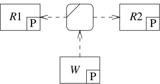
Now consider a program which receives events from two sensors (Figure 2.3). Inputs from Sensor 1 come every T1time units and each needs C1time units for computation;
events from Sensor 2 come every T2 time units and each needs C2 time units. Assume
the deadlines are the same as the periods, i.e. T1time units for Sensor 1 and T2time units
for Sensor 2. Under what conditions will these deadlines be met?
More generally, if a program receives events from n such devices, how can it be de-termined if the deadline for each device will be satisfied?
Before we begin to analyze this problem, we first define a program model and a sys-tem model. This allows us to study the problem of timing analysis in a limited context. We consider simple models in this chapter; more elaborate models will be considered in Chapters 3 and 4.
Program model
Assume that a real-time program consists of a number of independent tasks that do not share data or communicate with each other. A task is periodically invoked by the occur-rence of a particular event.
0
1 01
4T1
3T1
2T1
T2 2T2
sensor 1
sensor 2
T1
System model
Assume that the system has one processor; the system periodically receives events from the external environment and these are not buffered. Each event is an invocation for a particular task. Note that events may be periodically produced by the environment or the system may have a timer that periodically creates the events.
Let the tasks of program P beτ1;τ
2;:::;τn. Let the inter-arrival time, or period, for
invocations to taskτibe Tiand let the computation time for each such invocation be Ci. We shall use the following terminology:
A task is released when it has a waiting invocation.
A task is ready as long as the processing associated with an invocation has not been
completed.
A processor is idle when it is not executing a task.
2.2
Static scheduling
One way to schedule the program is to analyze its tasks statically and determine their timing properties. These times can be used to create a fixed scheduling table according to which tasks will be despatched for execution at run-time. Thus, the order of execution of tasks is fixed and it is assumed that their execution times are also fixed.
Typically, if tasksτ1;τ2;:::;τn have periods of T1;T2;:::;Tn, the table must cover
scheduling for a length of time equal to the least common multiple of the periods, i.e.
LCM(fT 1;T
2;:::;Tng), as that is the time in which each task will have an integral
num-ber of invocations. If any of the Ti are co-primes, this length of time can be extremely large so where possible it is advisable to choose values of Ti that are small multiples of a common value.
Static scheduling has the significant advantage that the order of execution of tasks is determined ‘off-line’, before the execution of the program, so the run-time scheduling overheads can be very small. But it has some major disadvantages:
There is no flexibility at run-time as all choices must be made in advance and must
therefore be made conservatively to cater for every possible demand for computa-tion.
It is difficult to cater for sporadic tasks which may occur occasionally, if ever, but
which have high urgency when they do occur.
0
1
overrun here
τ1
τ2
τ3
2 7 14
6 16
0 13
time
Figure 2.4 Priorities without pre-emption
2.3
Scheduling with priorities
In scheduling terms, a priority is usually a positive integer representing the urgency or importance assigned to an activity. By convention, the urgency is in inverse order to the numeric value of the priority and priority 1 is the highest level of priority. We shall assume here that a task has a single, fixed priority. Consider the following two simple scheduling disciplines:
Priority-based execution
When the processor is idle, the ready task with the highest priority is chosen for execu-tion; once chosen, a task is run to completion.
Pre-emptive priority-based execution
When the processor is idle, the ready task with the highest priority is chosen for execu-tion; at any time execution of a task can be pre-empted if a task of higher priority becomes ready. Thus, at all times the processor is either idle or executing the ready task with the highest priority.
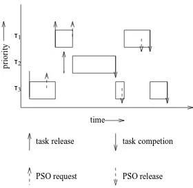
Example 2.1 Consider a program with 3 tasks, τ1,τ2 and τ3, that have the priorities, repetition periods and computation times defined in Figure 2.4. Let the deadline Di for each taskτibe Ti. Assume that the tasks are scheduled according to priorities, with no pre-emption.
Priority Period Comp.time
τ1 1 7 2
τ2 2 16 4
τ3 3 31 7
If all three tasks have invocations and are ready at time=0, taskτ1 will be chosen for
0
1
9
τ1
τ2
τ3
2 7 14
6 20
0 21
time
Figure 2.5 Priorities with pre-emption
At that time, only task τ3 is ready for execution and it will execute from time=6 to
time=13, even though an invocation comes for task τ1 at time=7. So there is just one unit of time for taskτ1to complete its computation requirement of two units and its next
invocation will arrive before processing of the previous invocation is complete.
In some cases, the priorities allotted to tasks can be used to solve such problems; in this case, there is no allocation of priorities to tasks under which task τ1 will meet its
deadlines. But a simple examination of the timing diagram shows that between time=15 and time=31 (at which the next invocation for task τ3 will arrive) the processor is not always busy and taskτ3does not need to complete its execution until time=31. If there were some way of making the processor available to tasksτ1 andτ2when needed and
then returning it to taskτ3, they could all meet their deadlines.
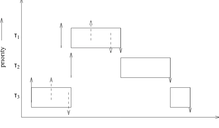
This can be done using priorities with pre-emption: execution of taskτ3 will then be
pre-empted at time=7, allowing taskτ1to complete its execution at time=9 (Figure 2.5). Processτ3 is pre-empted once more by taskτ1 at time=14 and this is followed by the next execution of task τ2 from time=16 to time=20 before taskτ3 completes the rest of
its execution at time=21.
2.4
Simple methods of analysis
Timing diagrams provide a good way to visualize and even to calculate the timing prop-erties of simple programs. But they have obvious limits, not least of which is that a very long sheet of paper might be needed to draw some timing diagrams! A better method of analysis would be to derive conditions to be satisfied by the timing properties of a pro-gram for it to meet its deadlines.
Using the notation of the previous section, in the following sections we shall consider a number of conditions that might be applied. We shall first examine conditions that are
necessary to ensure that an implementation is feasible. The aim is to find necessary
con-ditions that are also sufficient, so that if they are satisfied an implementation is guaranteed to be feasible.
2.4.1 Necessary conditions
Condition C1
8iCi < Ti
It is obviously necessary that the computation time for a task is smaller than its period, as, without this condition, its implementation can be trivially shown to be infeasible.
However, this condition is not sufficient, as can be seen from the following example.
Example 2.2
Priority Period Comp.time
τ1 1 10 8
τ2 2 5 3
At time=0, execution of taskτ1begins (since it has the higher priority) and this will
continue for eight time units before the processor is relinquished; taskτ2will therefore
miss its first deadline at time=5.
Thus, under Condition C1, it is possible that the total time needed for computation in an interval of time is larger than the length of the interval. The next condition seeks to remove this weakness.
Condition C2
i
∑
j=1
, Cj=T
j
1
Ci=T
iis the utilization of the processor in unit time at level i. Condition C2 improves on Condition C1 in an important way: not only is the utilization Ci=Tirequired to be less
than 1 but the sum of this ratio over all tasks is also required not to exceed 1. Thus, taken over a sufficiently long interval, the total time needed for computation must lie within that interval.
Example 2.3
Priority Period Comp.time
τ1 1 6 3
τ2 1 9 2
τ3 2 11 2
Exercise 2.4.1 Draw a timing diagram for Example 2.3 and show that the deadline for
τ3is not met.
Condition C2 checks that over an interval of time the arithmetic sum of the utilizations
Ci=Tiis 1. But that is not sufficient to ensure that the total computation time needed
for each task, and for all those of higher priority, is also smaller than the period of each task.
Condition C3
8i i,1
∑
j=1
Ti
Tj C
j
T i,C
i
Here, Condition C2 has been strengthened so that, for each task, account is taken of the computation needs of all higher priority tasks. Assume that Ti=Tjrepresents integer
division:
Processing of all invocations at priority levels 1:::i,1 must be completed in the
time Ti,C
i, as this is the ‘free’ time available at that level.
At each level j, 1ji,1, there will be Ti=Tjinvocations in the time Tiand each
invocation will need a computation time of Cj.
Hence, at level j the total computation time needed is
Ti
Tj Cj
and summing this over all values of j<i will give the total computation needed at level
i. Condition C3 says that this must be true for all values of i.
This is another necessary condition. But, once again, it is not sufficient: if Tj >Ti,
Condition C3 reduces to Condition C1 which has already been shown to be not sufficient. There is another problem with Condition C3. It assumes that there are Ti=Tj
invoca-tions at level j in the time Ti. If Tiis not exactly divisible by Tj, then eitherdTi=Tjeis an
overestimate of the number of invocations orbTi=Tjcis an underestimate. In both cases,
an exact condition will be hard to define.
To avoid the approximation resulting from integer division, consider an interval Mi which is the least common multiple of all periods up to Ti:
Mi=LCM(fT 1;T
2;:::;Tig)
Since Miis exactly divisible by all Tj;j<i, the number of invocations at any level j within
Miis exactly Mi=Mj.
Condition C4
i
∑
j=1
Cj
Mi=Tj
Mi
1
Condition C4 is the Load Relation and must be satisfied by any feasible implementa-tion. However, this condition averages the computational requirements over each LCM period and can easily be shown to be not sufficient.
Example 2.4
Priority Period Comp.time
τ1 1 12 5
τ2 2 4 2
Since the computation time of taskτ1exceeds the period of taskτ2, the implementation is infeasible, though it does satisfy Condition C4.
Condition C4 can, moreover, be simplified to
i
∑
j=1
, Cj=Tj
1
which is Condition 2 and thus is necessary but not sufficient.
Condition C2 fails to take account of an important requirement of any feasible imple-mentation. Not only must the average load be smaller than 1 over the interval Mi, but the load must at all times be sufficiently small for the deadlines to be met. More precisely, if at any time T there are t time units left for the next deadline at priority level i, the total computation requirement at time T for level i and all higher levels must be smaller than
t. Since it averages over the whole of the interval Mi, Condition C2 is unable to take account of peaks in the computational requirements.
But while on the one hand it is necessary that at every instant there is sufficient com-putation time remaining for all deadlines to be met, it is important to remember that once a deadline at level i has been met there is no further need to make provision for compu-tation at that level up to the end of the current period. Conditions which average over a long interval may take account of computations over the whole of that interval, includ-ing the time after a deadline has been met. For example, in Figure 2.5, taskτ2has met its
first deadline at time=6 and the computations at level 1 from time=7 to time=9 and from
time=14 to time=16 cannot affectτ2’s response time, even though they occur before the
end ofτ2’s period at time=16.
2.4.2 A sufficient condition
18
τ1
τ2
6 12
time
Figure 2.6 Timing diagram for Example 2.5
Consider, instead, assigning priorities to tasks in rate-monotonic order, i.e. in the inverse order to their repetition periods. Assume that task deadlines are the same as their peri-ods. It can then be shown that if under a rate-monotonic allocation an implementation is infeasible then it will be infeasible under all other similar allocations.
Let time=0 be a critical instant, when invocations to all tasks arrive simultaneously. For an implementation to be feasible, the following condition must hold.
Condition C5
The first deadline for every task must be met. This will occur if the following relation is satisfied:
n
21=n ,1
n
∑
i=1
Ci=T i
For n=2, the upper bound to the utilization∑ n i=1
Ci=Tiis 82:84%; for large values of n
the limit is 69:31%.
This bound is conservative: it is sufficient but not necessary. Consider the following example.
Example 2.5
Priority Period Comp.time
τ1 1 6 4
τ2 2 12 4
In this case (Figure 2.6), the utilisation is 100% and thus fails the test. On the other hand, it is quite clear from the graphical analysis that the implementation is feasible as all deadlines are met.
2.5
Exact analysis
time
Tj
t0
t j
Figure 2.7 Inputs([t;t 0
);j) =5
is feasible if at each priority level i, the worst-case response time riis less than or equal to the deadline Di. As before, we assume that the critical instant is at time=0.
If every taskτj, j<i, has higher priority thanτi, the worst-case response time Riis
Ri=Ci+ i,1
∑
j=1 d
Ri
Tj eCj
In this form, the equation is hard to solve (since Riappears on both sides).
2.5.1 Necessary and sufficient conditions
In this section, we show how response times can be calculated in a constructive way which illustrates how they are related to the number of invocations in an interval and the computation time needed for each invocation.
For the calculation, we shall make use of half-open intervals of the form[t;t 0
), t<t 0
, which contain all values from t up to, but not including, t0
. We first define a function Inputs([t;t
0
);j), whose value is the number of events at
pri-ority level j arriving in the half-open interval of time[t;t 0
)(see Figure 2.7):
Inputs([t;t 0
);j)= dt 0
=Tje,dt=Tje
The computation time needed for these invocations is
Inputs([t;t 0
);j)Cj
So, at level i the computation time needed for all invocations at levels higher than i can be defined by the function Comp([t;t
0 );i):
Comp([t;t 0
);i)= i,1
∑
j=1
Inputs([t;t 0
Let the response time at level i in the interval[t;t 0
)be the value of the function R(t;t 0
;i).
Let the computation time needed at level i in the interval[t;t 0
)be t 0
,t. The total
compu-tation time needed in this interval for all higher levels 0:::i,1 is Comp([t;t 0
);i); if this
is zero, the processor will not be pre-empted in the interval and the whole of the time will be available for use at level i. Now suppose that the total computation time needed in the interval for the higher levels is not zero, i.e. Comp([t;t
0
);i)>0. Then the response time
at level i cannot be less than t0
+Comp([t;t 0
);i). This can be generalized to the following
recursive definition of the function R(t;t 0
;i):
R(t;t 0
;i)= if Comp([t;t 0
);i)=0thent 0
elseR(t 0
;t 0
+Comp([t;t 0
);i);i)
Another way to explain this is to note that in the interval[t;t 0
), the computation still to
be completed at time t0
(which is just outside the interval) is
(t 0
,t),((t 0
,t),Comp([t;t 0
);i))=Comp([t;t 0
);i)
The value of the function R at level i is the time when there is no computation pending at level i or any higher level, i.e. Comp([t;t
0
);i)=0, and the whole of the interval[t;t 0
)
has been used for computation.
The worst-case response time at level i can then be defined as
Ri=R(0;C i;i)
If no computation is needed at levels 0:::i,1, then the response time at level i is
the computation time Ci; otherwise, add to Cithe amount of time needed at the higher levels. The object is to ‘push’ the estimated response time forward in decreasing jumps until eventually Comp([t;t
0
);i)=0. Computation of Riwill terminate, i.e. the jumps are
guaranteed to be diminishing, if the average load relation (Condition C4) is satisfied, i.e.
i
∑
j=1
Cj
Mi=Tj
Mi
1
2.5.2 Proof of correctness
We now show that the solution to the equation
Ri =Ci+ i,1
∑
j=1 d
Ri
Tj
eCj
given in terms of the function R is correct.
First observe that since the function Comp has been defined over intervals, there is some t2such that
Proof: Let the sum of the computation time needed in the interval [0;t) at the levels
0:::i,1 plus the time needed at level i be