Multiple Tracking of Moving Objects with Kalman
Filtering and PCA-GMM Method
Emadeldeen Noureldaim, Mohamed Jedra, Nouredine Zahid
Laboratory of Conception and Systems, Faculty of Sciences, Mohamed V University, Rabat, Morocco
Email: [email protected], [email protected], [email protected]
Received February 8, 2013; accepted March 11, 2013; accepted March 20, 2013
ABSTRACT
In this article we propose to combine an integrated method, the PCA-GMM method that generates a relatively improved segmentation outcome as compared to conventional GMM with Kalman Filtering (KF). The combined new method the PCA-GMM-KF attempts tracking multiple moving objects; the size and position of the objects along the sequence of their images in dynamic scenes. The obtained experimental results successfully illustrate the tracking of multiple mov-ing objects based on this robust combination
Keywords: Component; Pixels; Gaussian Mixture Model; Principle Component Analysis; Background Model;
Noise Process; Segmentation; Tracking; Kalman Filtering
1. Introduction
Object tracking is an important technique used in many systems, especially in the field of computer vision. Back- ground subtraction involves calculating the reference image and labeling the pixels corresponding to fore-ground objects. N. Friedman and S. Russell were pro-posed a Gaussian mixture model (GMM) for the back-ground subtraction [1]. C. Stauffer and W. Grimson de-veloped an algorithm for foreground segmentation based
on the Gaussian mixture model [2,3]. W. Grimson and et
al. used tracking information in multicamera calibration,
for object detection and classification [4]. T. Bouwmans, F. ElBaf and B. Vachon surveyed the background mod-eling using mixture of Gaussians for object detection [5]. F. Zbu and K. Fujimura demonstrated a face tracking method using GMM and EM algorithm [6]. P. Kaew-TraKulPong and R. Bowden proposed a method to detect moving shadows using Gaussian mixture model. The shadow detection also reduces the effect of small repeti-tive motions in the background scene [7]. On the other hand, the binding ellipsis, due to S. Cheung and C. Ka-math is inappropriate for complex-shaped objects such as human beings. They used frame-differencing as it pro-duces minimal false foreground trails behind objects [8]. R. Chan and J. Lin introduce mixture Kalman filtering for on-line estimation and prediction in conditional dy-namic linear model [9]. A. Yilmaz, O. Javed, and M. Shah surveyed detection of object and tracking [10]. K. Quast and A. Kaup presented Auto GMM-SAMT video
surveillance system and used the mean shift algorithm to track the contour of objects of changing shape without the help of any predefined shape model [11].
P. Sribi-Vasa proposed a new image segmentation algo-rithm used the finite mixture of doubly truncated bivari-ate Gaussian distribution by integrating this distribution with the hierarchical clustering [19]. K. Panta proposed novel data association schemes for the probability hypo- thesis density [20].
is a Gaussian probability density defined as follows:
In our work, we show that the segmentation of moving objects generated by PCA-GMM performed relatively better than the conventional GMM. This improvement in performance is based on the following: given that GMM segments the foreground from the background labeling for each sequence frame, where the background model can be updated using sufficient statistics and all the esti-mated parameter can be obtained efficiently. However, when the foreground is not available, or can be changed due to critical situations like illumination changes or it has been removed from the scene, then the GMM needs to consider such situations. The PCA-GMM is an exten-sion to GMM which considers these limitations [21]. The PCA-GMM which integrates PCA with GMM produces precise and clear features of the shape in the scenes and provides good classification of the object. The tracking of moving object is then based on applying KF on this integrated method.
The remainder of the paper is organized as follows: In the Section 2, we introduced the PCA-GMM that links GMM with PCA, followed by brief description of Kal-man filtering method, the experiment results of tracking moving objects by applying KF to PCA-GMM are placed in Section 4, followed by a conclusion in Section 5.
2. The PCA-GMM Method
First, in the adaptive mixture of Gaussian method, GMM, we considered the pixel processes as time series such that each pixel assumed to be an independent statistical proc- ess, incorporates all pixel observations. The mixture mo- del does not distinguish components that correspond to background from those associated with foreground ob- jects and record the observed intensity at each pixel over the previous N frames.
In the same manner as C. Stauffer and W. Grimson [3],
we used the same number k of components
K3,5
,
. We consider the values of a particular pixel, with initial
0 x y0 0
, :1
over time t and we can define the history of
this particular pixel as
1
X1, , Xt
I j j j t , where I is theimage sequence. The probability of pixels observation
data X is defined as follows:
t k 1 k Kp X
W
,t Xt,k t, ,
k t,,
k t
W kth
t
(1)
where is the weight of each component at
time , k t, is the mean and k t, is the covariance
mixture of each component at time t respectively,
th
k
, ,
T 1
, , ,
1 2 2
, , 1
exp 2π
t k t k t
t k t k t t k t n
k
X
X X
2
(2)
For simplicity we use k t, kI
,
W
, where I is the
iden-tity matrix. Next, we update the mixture of each pixel consecutively by reading in new pixel values and update each matching mixture component. We initialize the
pa-rameters and . They are updated for each
frame in the mixture. We calculate W for each Gaussian component in the mixture. When the current pixel value matches none of the distributions, the least probable distribution is updated with the current pixel values. Then the parameters of the mixture are updated as follows:
th
k
, 1 , 1 ,
k t k t k t
W W M (3)
where the constant is a learning rate to update the
components weights, Mk t, is a dummy variable with
value 1 for matching models and 0 otherwise. We intro-duce the following criterion for screening the preliminary Gaussian matching distribution with Mahalanobis
dis-tance less than a threshold T
12 ,
min
k
t k t
X T (4)
to collect the targeted pixels, with the update recursive equations
, 1 , 1 ,
k t p k t p Xk t
T
2 2
, , 1 , , , ,
1
1 K
k t k t k t k t k t k t
k
p p X X
(5)
and
(6)
where p Xt t, t
indicates how to acceleratethe update. Thus, we can find the foreground resulted from the background and then find the best segment of the image. The non active background Gaussian is treated as foreground. In the ordering, we selected the
ratios Wk k Large values of ratios are associated with
distributions which have a high weight, low variance.
The first B distributions chosen under the expression:
3, 1
arg minb b k t
k
B W T
(7)
where the threshold T is a prior probability estimated
from the background process. Movements caused by the background (such as tree branches shaking, surface fluc-tuations, etc.) were considered to segment for the fore-ground objects.
X
, 1, ,S St t N we propose to compute
we consider each of the N frames in one color R
i
th
j
, 1
j i N
th i
such that we can define the frame vectors for fixed with
respect to the pixels index:
,
i i
R r , , (8)
The arithmetic average of pixels in each component
for the frame vector can be defined as follows:
, 1 i N j
1i i j
i r r N N (9)
where i is number of pixels in the frame i. Next, we
compute the difference i i i for the image
and construct the difference matrix R r A as:
ith
i
1, , N
A The covariance matrix of each
frame vector is defined by:
T 1 N T
i i i N V V 1
AA (10)
We compute the eigenvectors and corresponding ei-genvalues by:
S
(11) using Singular Value Decomposition (SVD) method,
where V is the set of eigenvectors associated with the
corresponding eigenvalues λ. To apply the method of
PCA we need to define the projection i by applying
the translation matrix VT to the vectors
i i
X r as follows:
T
i i i
S V r
ˆi
X (12)
Next, we construct each frame to obtain the features of
the shape. Then we can define the estimated data x by:
ˆi i
x V S r (13) One property of PCA is that the projection onto the prin-cipal subspace minimizes squared errors. To find the feature principal subspecies of PCA, the sequential re-construction errors are estimated from:
2 1 N i i ˆ i X x
i (14)the major advantage of the PCA method comes from its generalization ability. It reduces the feature space dimen-sion by considering the variance of the input data. This method determines which projections are preferable for representing the structure of input data. Those projec-tions are selected in such a way that the maximum
amount of information (i.e. maximum values of variances,
where Eigenvalues represent the largest variances) is obtained in the smallest dimension of feature space.
The PCA-GMM addresses the major limitation of the GMM, which is the illumination changes and noise. The
PCA-GMM method considers observing pixel data X
from (1, 2), using the method of PCA. The estimated xˆ
is obtained by projecting the data on the axis, then with
the new data
tp X
,
, ,
1ˆ
, ,ˆ
K
t k t t k t k t
k
p S W S
based on S such that:
(15)
T 1
, , 1 , , ,
2 2
1 ˆ
, ,ˆ e px
2π
t k t k t n k t k t k t
S S S
2 ˆ ˆ (16)
and again for simplicity we assume k t, k t,I
p S
, where I
is identity matrix. In linking PCA with GMM it is
evi-dent that the integrated t based on S
t byits physical structure, contains the maximum amount of information or has the minimum squared errors as com-pared to
S
p Xt based on X
Xt
ˆ
of the GMM in handling the limitation and shadow that contribute to noise in the adaptive Gaussian model.
To update each mixture of each pixel entails reading the new pixel values and select the matching components,
then compute the mean obtained with x and finally
injecting that mean into the covariance of PCA method form (5, 6). Symbolically the update is based on:
, , 1 ,
ˆk t 1 p ˆk t p xˆk t
T
2 2
, , 1 , , , ,
1
ˆk t 1 ˆk t K k t ˆk t k t ˆk t k
p p S S
(17) and (18)
where p St ˆ ˆt, t
ˆ
indicates how to accelerate the update. In the integrated method we insert the
esti-mates of the mean i t, and covariance i t, of each
component in PCA into GMM respectively. We simply select the components with largest weights and re-esti- mate with (7) as follows:
ˆ
, , 1 ,
ˆ 1 ˆ ˆ
k t k t k t
W W M (19)
And their Gaussian matching parameters must satisfy:
1
, 2
, ˆ ,
min
k t
k t k t
S T (20)
ˆ ˆ
k k
W
with the estimates of the ratios . The large values
of ratios are associated with distributions which have a high weights or low variances. We select the first Gaussian distributions:
ˆ
B
3 , 1ˆ arg min b ˆ
b k t k
B W T
manipulation. (21) 3. Kalman Filtering: The Version of
A estimate the state of a
t
PCA-GMM-KF Method
Kalman Filter (KF) is applied to
linear system where the state is assumed to be Gaussian distributed. This filter not only provides an efficient computational solution to sequential systems but also provides an optimal solution for the discrete data for lin-ear filtering problem [22]. On tracking objects from frame to frame in long sequences of images, the continu-ity of the motion of the observed scene, allows the pre-diction of the image, at any instant, based on their previ-ous trajectories. Because the moving state changes little in the neighboring consecutive frames, we model the system as linear Gaussian with the state parameters of Kalman filter given by the object location, its velocity and its size of the object respectively. A discrete-time dynamic equation state is given by
t1 t t
X X s (22)
where the state vector X
x y u v, , , , ,
T1 0 0 0 0 1 0 0 1 0 0 0 1 1 0 0 0 0 0 1
,
t , 1
0
0 1 0 0 0 0 0 0
x and y are the predicted coordinates of the object,
u and are velocities in respective direction, v
present he width of the object rectangle, t
re t repr
-sents the change in time t and, t
e
s is the white
Gaus-sian noise with zero means and c variance matrix Qt,
that is t
0, t
o
s N Q . The position of obtained PCA-
GMM algorithm will be the measurement vector Zt.that
can be injected in the measurement model of KF. Ac-cordantly:
t t t t
Z H X q (23)
Equation (23) combines PCA-GMM co
with KF. Such a mbination proposes what we may call PCA-GMM-KF, as a version of Kalman Filtering in tracking multiple
moving objects. The predicted coordinates
x y, anddimensions ω of the rectangle in the measurem odel
of Equation (23) under PCA-GMM-KF are used to locate the object in the present frame. Where,
ent m
0,
t t
q N R is
white Gaussian noise, Rt is covariance matrix and Ht
is the design matrix such that
1 0 1
0 0 0
0 1 0 0 0 0 0 0 1
.
The corresponding cova atrices Qt1
0 1 0
t
H
riance m and
R imat1
are the inputs to the Kalman filter. In the sequential ge, if the dynamics of the moving object is known,
prediction can be made about the positions of the objects in the current image. The Kalman filter state prediction
t
X and state covariance prediction Pt are defined by:
1 1
t t ˆt
X X (24)
T
1ˆ 1 1 1
t t t t t
P P Q
where ˆt
(25)
and Pˆt denotes the estimat
X ed state vector
and error covariance matrix respectively at time t. Then
the Kalman filter update steps are as follows:
1T T
t t t t t t t
K P H H P H R (26)
ˆ
t t t t t t
X X K Z H X (27)
ˆ
t t t t
P I K H P (28)
KF algorithm starts with initial conditions with K0
and P0. Kt is the Kalman gain, which defines the
up-datin ht between the new measurements and the
prediction from the dynamic model. g weig
4. Experimental Results and Analysis
, in our
mentation using the G
sults based on PCA-GMM- K
by performing the fo
To demonstrate the effectiveness of the algorithm application, we first show how the PCA-GMM out-per- forms the conventional GMM algorithm. In our experi- ment, each pixel is checked against the current frame of the background model by comparing it with every com- ponent in the PCA-GMM. This relatively better per- formance of PCA-GMM is mainly due to its ability to manipulate the variation to ease the segmentation of the foreground from the background. Moreover, the PCA- GMM method is based on the minimum reconstruction error over the data needed to be estimated which contrib-ute for the better segmentation [22].
It is evident from viewing the seg
MM (Figure 1(a)), we can achieve remarkable
im-prove by using the segmentation on PCA-GMM (Figure
1(b)). Next, based on this segmentation result we are
motivated to tackle the tracking problem based on PCA- GMM rather than the GMM.
The tracking experimental re
F method, are arranged into two cases of tracking mul-tiple moving objects, where we have constructed two frame’s sequences in the different backgrounds. The frame’s dimensions were 167 × 120.
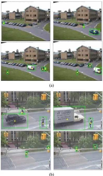
The tracking algorithm represented
llowing: First we apply the PCA-GMM algorithm to extract the moving objects from background in each video frame, and then we predict the next position can-didates in the next frame by predicting it from KF in Equations (22) and (23). Sequentially the tracking results based on the routine loop of detecting the objects by us-ing data association function and the add new hypotheses
function inKF algorithm respectively and finely we
in turn provides new input. Consequently, the resulted PCA-GMM-KF method reflects more accurate detection of object results at each level of the proposed approach (Figures 2(a) and (b)).
) (a
)
Figure 1. (a) Segmentation oving objects under tradi-(b
of m
tional GMM algorithm; (b) Segmentation of moving object under PCA-GMM algorithm.
(a)
(
Figure 2. Tracking of mul moving objects based on PCA-GMM-KF.
on
ttempt to improve tracking of multiple
[1] N. Friedman e Segmentation in
Video Sequences: A Probabilistic Approach,” The 13th
Proceedings of
e Tracking,” IEEE Transactions on
b)
tiple
After we applied the PCA to solve the problem of Gaussian mixture and obtained improved result in the
two cases: (Figures 2(a) and (b)), the performance
en-hanced remarkably with the PCA-GMM proposed detec-tion method.
5. Conclusi
In this article, we a
moving objects within the framework of Kalman Filter-ing. Given that the integrated combined PCA-GMM outperforms the conventional GMM in generating rela-tively improved performance in segmentation, we have been motivated to address the tracking of multiple ob-jects within the framework of KF. The experimental re-sults in addition of illustrating the outperformance of segmentation results of the PCA-GMM algorithm over GMM, have also considered the tracking of multiple mo- ving objects. The proposed PCA-GMM-KF method which utilized the desirable segmentation results due to PCA- GMM can be viewed as a version of KF. The experi-mental results of tracking objects have shown that that the application of PCA-GMM-KF method to each case and under sequence of images, successfully captured the objects and produces a satisfactory results.
REFERENCES
and S. Russell, “ImagConference on Uncertainty in Artificial Intelligence, Brown University, Rhode Island, Morgan Kaufmann Publishers, Inc., San Francisco, 1997, pp. 175-181.
[2] C. Stauffer and W. Grimson “Adaptive Background Mix-ture Models for Real-Time Tracking,”
IEEE Computer Vision and Pattern Recognition, Vol. 2, 1999, pp. 246-252.
[3] C. Stauffer and W. Grimson, “Learning Patterns of Activ-ity Using Real-Tim
Pattern Analysis & Machine Intelligence, Vol. 22, No. 8, 2000, pp. 747-757. doi:10.1109/34.868677
[4] W. Grimson, C. Stauffer, R. Romano and L. Lee, “Using Adaptive Tracking to Classify and Monitor Activities in a
g Using Mixture of Gaussians for Foreground
GMM),” Proceedings of IEEE
Site,” Proceedings of IEEE Computer Society Conference on Computer Vision and Pattern Recognition, 1998, pp. 22-29.
[5] T. Bouwmans, F. El Baf and B. Vachon, “Background Modelin
Detection,” Recent Patents on Computer Science, Vol. 1, No. 3, 2008, pp. 219-237.
[6] Y. Zhu and K. Fujimura, “Driver Face Tracking Using Gaussian Mixture model (
on Intelligent Vehicles Symposium, OH, 2003, pp. 587- 592. doi:10.1109/IVS.2003.1212978
[image:5.595.73.271.369.708.2]P Journal on Applied Signal Processing Advanced Video Based Surveillance Systems, September 2001.
[8] S. Cheung and C. Kamath, “Robust Background Subtrac-tion with Foreground ValidaSubtrac-tion for Urban Traffic Vi-
deo,” EURASI ,
Vol. 14, 2005, pp. 2330-2340. doi:10.1155/ASP.2005.2330
[9] R. Chen and J. S. Liu, “Mixture Kalman Filters,” Journal of the Royal Statistical Society
thodology, Vol. 62, No. 3, 2000, pp. 493-508. , Series B-Statistical Me-doi:10.1111/1467-9868.00246
[10] A. Yilmaz, O. Javed and M. Shah, “Object Tracking: A Survey,” ACM Computing Surveys, Vol. 38, N
pp. 1-45.
o. 4, 1177355
2006, doi:10.1145/1177352.
Image and
Vi-1. [11] K. Quast and A. Kaup, “AUTO GMM-SAMT: An
Auto-matic Object Tracking System for Video Surveillance in Traffic Scenarios,” EURASIP Journal on
deo Processing, Vol. 2011, No. 1, 2011, pp. 2-14. [12] H. Moon and P. Jonathan, “Computational and
Perform-ance Aspects of PCA-Based Face-Recognition Algori- thms,” Perception, Vol. 30, No. 3, 2001, pp. 303-32 doi:10.1068/p2896
[13] H. Kim, D. Kim and S. Yang, “An Efficient Model Order Selection for PCA Mixture Model,” Pattern Recogniti
Vol. 24, No. 9-10, 2
on
003, pp. 1385-1393.
,
doi:10.1016/S0167-8655(02)00379-3
[14] B. Antoni, M. Vijay and V. Nuno, “Generalized Stauffer- Grimson Background Subtraction for Dy
Journal of Machine Vision and Applicationsnamic Scenes,” , Vol. 22, No. 5, 2011, pp. 751-766.
[15] I. Gómez, D. Olivieri, X. Vila and S. Orozco, “Simple Human Gesture Detection and Recognition Using a
Fea-ture Vector and a Real-Time Histogram Based Algo-rithm,” Journal of Signal and Information Processing, Vol. 2, No. 4, 2011, pp. 279-286.
doi:10.4236/jsip.2011.24040
[16] Y. Sheikh and M. Shah, “Bayesian Modeling of Dynamic Scenes for Object Detection,” IEEE Transactions on Pat-tern Analysis and Machine Intelligence, Vol. 27, No. 1, 2005, pp. 1778-1792. doi:10.1109/TPAMI.2005.213 [17] Y. Yong and W. Ya-Fei, “Moving Object Detection Ba-
Wong, “Adaptive
a, “Image
chemes for the Prob-sed on Spatial Local Correlation,” Opto-Electronic Engi-neering, Vol. 36, No. 2, 2009, pp. 1-5.
[18] R. Hassanpour, A. Shahbahrami and S.
Gaussian Mixture Model for Skin Color Segmentation,”
Proceeding of World Academic of Science Engineering and Technology, Vol. 31, 2008, pp.1307-6884.
[19] G. Rajkumar, K. Srinivasarho and P. Sribivas
Segmentation Method Based on Finite Doubly Truncated Bivariate Gaussian Mixture Model with Hierarchical Clus- tering,” International Journal of Computer Science Issues, Vol. 8, No. 2, 2011, pp. 1694-0814.
[20] K. Panta, “Novel Data Association S
ability Hypothesis Density Filter,” IEEE Transactions on Aerospace and Electronic Systems, Vol. 43, No. 2, 2007, pp. 556-570. doi:10.1109/TAES.2007.4285353
[21] N. Emadeldeen, M. Jedra and N. Zahid, “On Segmenta-tion of Moving Objects by Integrating PCA Method with the Adaptive Background Model,” Journal of Signal and Information Processing, Vol. 3, No. 3, 2012, pp. 387-393. doi:10.4236/jsip.2012.33051