Abstract—In this paper, we present a preliminary study of the formulation of two new explicit group relaxation methods for the difference solution of the two dimensional second order hyperbolic telegraph equations. The methods are derived from the standard centred and rotated five-point finite difference discretisations. Their computational complexity analysis is discussed. Numerical experimentations are also conducted to demonstrate the viability of the explicit group formulations.
Index Terms—computational complexity analysis, finite difference method, group explicit method, telegraph equations.
I. INTRODUCTION
Explicit group methods for solving the two dimensional elliptic and parabolic equations using finite difference schemes have been extensively investigated over the years [1]-[6]. The advantages of using these methods are easier implementation and lesser execution timings requirements than the point iterative methods. These methods are also favorable in parallelism due to their explicit nature.
In recent years, numerous methods have been introduced in the literature for numerical solution of one- and two- dimensional hyperbolic equations [7]-[15]. In particular [10], an implicit three-level scheme was developed by Mohanty while Evans [7] implemented explicit group methods for the nonlinear convection equation.
In this paper, we introduce new explicit group methods for the solution of the two dimensional second order hyperbolic equation which is commonly encountered in physics and engineering mathematics. In the next section, we will give an overview of the formulation of the explicit group methods followed by the computational complexity analysis in Section III. The numerical experiments and the results are presented in Section IV. Finally, concluding remarks is given in Section V.
II. THE GROUP ITERATIVE METHODS
In this section, we briefly introduce the explicit group methods for the two dimensional second order hyperbolic equations based on two finite difference approximations,
Manuscript received March 1, 2010. This research was supported by the Universiti Sains Malaysia Research University Grant (1001/PMATHS/817027).
Kew Lee Ming is a doctoral candidate at the School of Mathematical Sciences, Universiti Sains Malaysia, 11800 Penang, Malaysia (corresponding author e-mail: [email protected]).
Norhashidah Hj. M. Ali is a permanent staff of School of Mathematical
specifically the standard and the rotated point iterative approximations.
Consider the two dimensional second order hyperbolic equation (telegraph equation) defined in the region
( , , ) | 0x y t x y, 1,t 0
of the following form: 2
2 2
2 2
2 2
2 ( , , ) ( , , )
( , , ) ( , , ) ( , , )
U U
x y t x y t U
t t
U U
A x y t B x y t F x y t
x y
(1)
where( , , )x y t 0,( , , )x y t 0, ( , , )A x y t 0, ( , , )B x y t 0. The initial and boundary conditions are given by
1 2
1 2
3 4
( , , 0) ( , ); ( , , 0) ( , )
(0, , ) ( , ); (1, , ) ( , ); ( , 0, ) ( , ); ( ,1, ) ( , ).
U
U x y f x y x y f x y
t
U y t g y t U y t g y t
U x t g x t U x t g x t
Let k 0 and h0 be the time step and space step respectively. We divide the interval 0x y, 1into (N1)
subinterval, so that (N1)h1.The grid points are given by ( ,x y ti j, m)( ,ih jh mk, )wherem1, 2, 3, ....
Standard Point Iterative Method
Finite difference discretisation of (1) using the common centred difference formula for the second partial derivatives will produce
, , 1 , , , , 1 , , 1 , , 1 2
1, , 1 , , 1 1, , 1 1, , , , 1, ,
2 2
, 1, 1 , , 1 , 1, 1 , 1, , , , 1,
2 2
2 2
2 2
2 2
1
2
2 2
1
2
( 2
i j m i j m i j m i j m i j m
i j m i j m i j m i j m i j m i j m
i j m i j m i j m i j m i j m i j m
u u u u u
u u u u u u
u u u u u u
t t
x x
y y
, , 1 , , 1
, , 2 )
i j m i j m i j m
u u F
(2)
where
1 ...
, , ; ( , 0,1, 2, ...,n ; 0,1, )
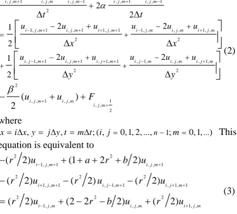
x i x y j y t m t i j m This equation is equivalent to
2 2
1, , 1 , , 1
2 2 2
1, , 1 , 1, 1 , 1, 1
2 2 2
1, , , , 1, ,
2 2 2
, 1, , 1, , , 1 , , 1/ 2
( 2) (1 2 2)
( 2) ( 2) ( 2)
( 2) (2 2 2) ( 2)
( 2) ( 2) ( 1)
i j m i j m
i j m i j m i j m
i j m i j m i j m
i j m i j m i j m i j m
r u a r b u
r u r u r u
r u r b u r u
r u r u a u t F
(3)
whereh x y 1 nand 2 2
, ,
r t h a t b t .
Explicit Group Iterative Methods for the
Solution of Telegraph Equations
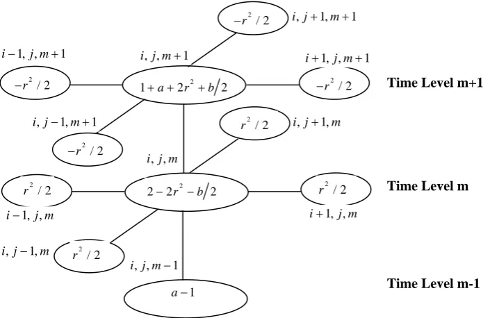
[image:1.595.307.549.505.723.2]Fig 1 Computational molecule of the standard point approximation (3)
Fig 2 Computational molecule of the rotated point approximation (5)
2 1 a 2r b 2
2 22r b 2
2 / 2 r
2 / 2 r
2 / 2 r
2 / 2 r
2 / 2 r
2 / 2 r 2
/ 2 r
1 a
Time Level m+1
Time Level m
Time Level m-1
, 1, 1
i j m
, , 1
i j m i1, ,j m1
1, , 1
i j m
, 1, 1
i j m i j, 1,m
, , i j m
1, , i j m 1, ,
i j m
, 1, i j m
, , 1
i j m 2
/ 2 r
Time Level m+1
Time Level m
Time Level m-1
, , 1
i j m
, , i j m
, , 1
i j m 2 1 a r b 2
2 2r b 2
1 a 2
/ 4 r
r2/ 4
2 / 4 r
2
/ 4 r 2
/ 4 r
2 / 4 r
2 / 4
r 2
/ 4 r
1, 1, 1
i j m
1, 1, 1
i j m
1, 1, 1
i j m
1, 1, 1
i j m
1, 1, i j m
1, 1, i j m
1, 1, i j m 1, 1,
Rotated Point Iterative Method
Using the rotated finite difference approximation (which is obtained by rotating the x-y axis clockwise 45 degrees) for the second partial derivatives, equation (1) becomes
, , 1 , , , , 1 , , 1 , , 1 2
1, 1, 1 , , 1 1, 1, 1 1, 1, , , 1, 1,
2 2
1, 1, 1 , , 1 1, 1, 1 1, 1, , , 1, 2 2 2 2 2 2 1
2 2 2
2 2
1
2 2
i j m i j m i j m i j m i j m
i j m i j m i j m i j m i j m i j m
i j m i j m i j m i j m i j m i
u u u u u
u u u u u
u u u u u
t t u x x u y
2 1, 2, , 1 , , 1
, , 2 2 2 ( ) j m
i j m i j m i j m
u u y F
(4)Upon simplification, the following is obtained
2 2
1, 1, 1 , , 1
2 2 2
1, 1, 1 1, 1, 1 1, 1, 1
2 2 2
1, 1, , , 1, 1,
2 2 2
1, 1, 1, 1, ( 1) , , 1 , , 1/ 2
( 4) (1 2)
( 4) ( 4) ( 4)
( 4) (2 2) ( 4)
( 4) ( 4)
i j m i j m
i j m i j m i j m
i j m i j m i j m
i j m i j m a i j m Fi j m
r u a r b u
r u r u r u
r u r b u r u
r u r u u t
[image:3.595.301.553.386.719.2] (5)
Fig 2 represents the computational molecule of the rotated point approximation (5). A point iterative scheme based on the by constructing 2 types of points on the x-y plane of the solution domain. We may then choose to iterate on one type of points and after convergence is achieved, the solutions at the remaining points will be evaluated directly using equation (3).
Explicit Group (EG) Iterative Method
Consider the standard point approximation which was derived from the central finite difference discretisation (2)-(3). Applying equation (3) to any group of four points on a discretised solution domain will result in a (4x4) system of equation as follows:
, , 1 ,
1, , 1 ,
1, 1, 1 1, 1
, 1, 1 , 1
1 2 3 2
2 1 2 3
3 2 1 2
2 3 2 1
i j m i j i j m i j i j m i j i j m i j
k k k k
k k k k
k k k k
k k k k
u rhs u rhs u rhs u rhs
(6) where 2 21 1 2 2 ; 2 2
k a r b k r and 3k 0
2 2
, 1, , 1 , 1, 1
2
1, , , 1, 1, , , 1, 2 , , , , 1 , , 1/ 2
(2 2 2) ( 1)
( 2)[ ]
( 2)[ ]
i j i j m i j m
i j m i j m i j m i j m i j m i j m i j m
r b a
rhs r u u
r u u u u
u u t F
2 2
1, 1, 1, 1 2 , , 1 2
, , 1, 1, 2 , , 1, 1, 2
1, , 1, , 1 1, , 1/ 2
(2 2 2) ( 1)
( 2)[ ]
( 2)[ ]
i j i j m i j m
i j m i j m i j m i j m i j m i j m i j m
r b a
rhs r u u
r u u u u
u u t F
2
1, 1 2 , 1, 1 1, 2 , 1 2
( 2)[ ]
( 2)[ ]
i j i j m i j m
rhs r u u
r u u u u
2 2
, 1 1, 1, 1 , 2 , 1 2
1, 1, , , 1, 1, , 2 , 2
, 1, , 1, 1 , 1, 1/ 2
(2 2 2) ( 1)
( 2) [ ]
( 2 [) ]
i j i j m i j m
i j m i j m i j m i j m i j m i j m i j m
r b a
rhs r u u
r u u u u
u u t F
The (4x4) system in (6) can be inverted to become
, , 1 ,
1, , 1 1,
1, 1, 1 1, 1
, 1, 1 , 1
1 2 3 2
2 1 2 3
3 2 1 2
2 3 2 1
i j m i j
i j m i j
i j m i j
i j m i j
m m m m
m m m m
m m m m
m m m m
u rhs u rhs u rhs u rhs
(7) where2 2 2 2 4 2
3 2 2 2 2 4 2 2
2 2 2 2 3 4 4 6 2 2
2 2 2 4 2 2 2
1 2(4 4 16 8 16 4 8 4 14 )
/(8 12 48 24 24 88 96 48 24 8
6 12 12 48 88 44 48 48 6 );
2 2 / (4 4 16 8 4 12 16 8 4 );
m a ab ar a r r b b r b
a a b a r a ab ar ar ar b a
ab b r b r b r r b r r b b
m r a ab ar a b r r r b b
m
4 3 2 2 2 2 4 2
2 2 2 2 2 3 4
4 6 2 2
3 4 / (8 12 48 24 24 88 96
48 24 6 12 12 8 48 88
44 48 48 6 ).
r a a b a r a ab ar ar
ar b a ab r b b r b r
r b r r b b
Explicit De-Coupled Group (EDG) Iterative Method
Similarly, applying equation (5) to any group of four points of the solution domain will result in (4x4) system of equations
, , 1 ,
1, 1, 1 1, 1
1, , 1 1,
, 1, 1 , 1
1 2 3 3
2 1 3 3
3 3 1 2
3 3 2 1
i j m i j i j m i j i j m i j i j m i j
k k k k
k k k k
k k k k
k k k k
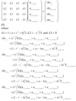
u rhs u rhs u rhs u rhs
(8) where 2 21 1 2 ; 2 4
k a r b k r and 3k 0
2 2
, 1, 1, 1 1, 1, 1 1, 1, 1 2
1, 1, 1, 1, 1, 1, 1, 1, 2 , , , , 1 , , 1/ 2
(2 2) ( 1)
( 4) [ ]
( 4)[ ]
i j i j m i j m i j m i j m i j m i j m i j m
i j m i j m i j m
r b a
rhs r u u u
r u u u u
u u t F
2 2
1, 1 2 , , 1 2 , 2 , 1 , 2 , 1 2
, , 2 , , 2 , 2, , 2 , 2
1, 1, 1, 1, 1 1, 1, 1/ 2 (
(2 2) ( 1)
4)[ ]
( 4)[ ]
i j i j m i j m i j m i j m i j m i j m i j m
i j m i j m i j m
r b a
rhs r u u u
r u u u u
u u t F
2 2
1, , 1, 1 2 , 1, 1 2 , 1, 1 2
, 1, 2 , 1, 2 , 1, , 1, 2
1, , 1, , 1 1, , 1/ 2 (
(2 2) ( 1)
4)[ ]
( 4) [ ]
i j i j m i j m i j m i j m i j m i j m i j m
i j m i j m i j m
r b a
rhs r u u u
r u u u u
u u t F
2 2
, 1 1, , 1 1, 2 , 1 1, 2 , 1 2
1, , 1, , 1, 2 , 1, 2 , 2
, 1, , 1, 1 , 1, 1/ 2
(2 2) ( 1)
( 4)[ ]
( 4)[ ]
i j i j m i j m i j m i j m i j m i j m i j m
i j m i j m i j m
r b a
rhs r u u u
r u u u u
u u t F
, , 1 ,
1, 1, 1 1, 1
1 2
1
2 1
i j m i j
i j m i j
m m
m m
A
u rhs
u rhs
(9) and1, , 1 1,
, 1, 1 , 1
1 2
1
2 1
i j m i j
i j m i j
m m
m m
A
u rhs
u rhs
(10) where
2 2 2 4 2 2
2 2
16 32 32 16 16 32 16 15 16 4
8(2 2 2
1 ;
;
4 . ) 2
a r b a ar ab r r b b
a r b
m m
A
r
The EDG scheme corresponds to generation of iterations on one type of points using equation (9) until a certain convergence criteria are met. After convergence is achieved, the solutions at the remaining points are evaluated directly once using the centred difference formula (3). The convergence of this scheme may be further accelerated by applying the SuccessiveOverRelaxation iterative scheme on the iterative formula.
III. COMPUTATIONAL COMPLEXITY ANALYSIS
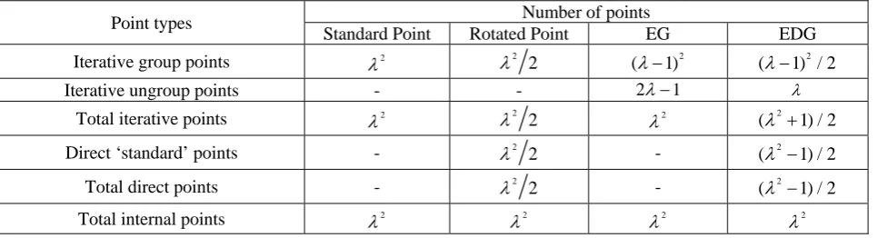
In this section, we analyze the computational complexity for the two explicit group methods and also for the standard and rotated point iterative methods. The estimation on this computational complexity is based on the arithmetic operations performed per iteration. Assume that the solution domain is discretised with grid size n, then the number of internal mesh points is given by 2 where n 1. Iterative points and direct points are two main types of internal mesh points. Iterative points are the points that are involved in the iteration process only, while the direct points are the points that are computed directly once using the standard difference formula after the iteration process achieves convergence. Table 1 lists the number of various mesh points for the point and explicit group methods. Table 2 shows the number of arithmetic operations required per iteration and the direct solution after convergence for each
method (excluding the convergence test). To further understand the complexity analysis of the group methods, please refer to [1] and [6].
IV. EXPERIMENTS AND DISCUSSION OF RESULTS
In order to verify the applicability of the proposed methods in solving the two dimensional second order hyperbolic equations, experiments were carried out on a PC with Core 2 Duo 2.8 GHz, 2GB of RAM with Window XP SP3 operating system using Cygwin C. All the four methods described in Sections II-III were applied to the model problem (1) with Dirichlet boundary conditions satisfying several exact solutions as listed in Table 3.
The methods were run using several mesh sizes of 10, 20, 50 and 98. For convenience, the relaxation factor
eis set [image:4.595.59.542.574.705.2]equal to 1.0 (Gauss-Seidel relaxation scheme). The convergence criteria used was the
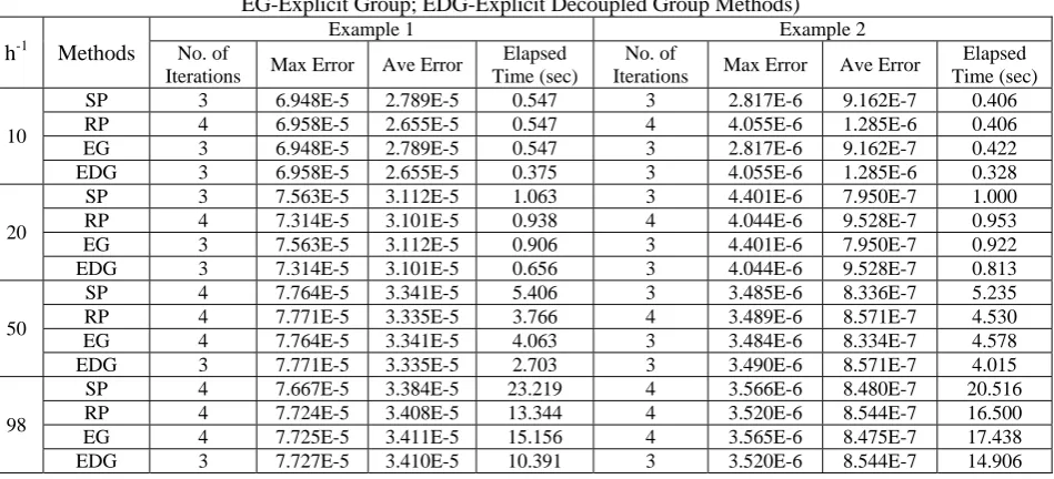
norm with the error tolerance set equal to 1010. The chosen time step for examples 1 and 2 was t 0.001 while t 0.1 was applied to example 3. Table 4 depicts the numerical results for the group relaxation methods described in Section II where the results are compared with the standard and rotated point iterative methods. Amongst the point methods, the rotated scheme is faster than the standard centred difference scheme as the grid size increases due to its lower computational complexities. It can be observed that the accuracies of the explicit group methods are as good as the standard and rotated point iterative methods but they require lesser computing timings to achieve the results. For example, the execution times of EDG is only about 44-68%, 72-81% and 16-34% of those of the standard centred point method in Examples 1, 2 and 3 respectively. From Table 2, it is clear that the theoretical computational costs for the group methods are lesser than the point methods with EDG requiring the least computing effort amongst the four methods.Table 1 Number of different types of mesh points in the point and explicit group methods
Point types Number of points
Standard Point Rotated Point EG EDG
Iterative group points 2 2
2
2
(1) (1) / 22
Iterative ungroup points - - 21
Total iterative points 2 2
2
2 2
( 1) / 2
Direct ‘standard’ points - 2
2
- 2
( 1) / 2
Total direct points - 2
2
- 2
( 1) / 2
Table 2 Computational complexity for the point and explicit group methods
Methods Per Iteration After Convergence
Additional Multiplication Additional Multiplication
Standard Point 2
12 52 - -
Rotated Point 2
6 52 2 2
6 52 2
EG 2
13(1) 12(21) 8(1)25(21) - -
EDG 2
[image:5.595.61.537.212.406.2]6(1) 12 7(1) / 22 5 6(21) 5(21) / 2
Table 3 Several examples with Dirichlet boundary conditions (Examples 1&2 [13]; Example 3 [14])
Exam -ples
Analytical solution Initial Condition Boundary Condition f x y t( , , )
1 2 2
( , , )
u x y t x y t 2 2
2 2
( , , 0) ,
( , , 0) 1.
t
u x y x y
u x y x y
2 2 2 2
(0, , ) ,
(1, , ) 1 ,
( , 0, ) ,
( ,1, ) 1 .
u y t y t
u y t y t
u x t x t
u x t x t
2 2 ( , , ) 2
f x y t x y t
2
( , , ) tsin( ) sin( )
u x y t e x y ( , , 0) sin( ) sin( ), ( , , 0) sin( ) sin( ).
t
u x y x y
u x y x y
(0, , ) ( , 0, ) 0, (1, , ) sin(1) sin( ), ( ,1, ) sin( ) sin(1).
t
t
u y t u x t
u y t e y
u x t e x
( , , ) 2 tsin( ) sin( )
f x y t e x y
3 u x y t( , , )log(1 x y t) ( , , 0) log(1 ), 1
( , , 0) .
1
t
u x y x y
u x y
x y
(0, , ) log(1 ), (1, , ) log(2 ), ( , 0, ) log(1 ), ( ,1, ) log(2 ).
u y t y t
u y t y t
u x t x t
u x t x t
2
( , , ) 2 (1 )
log(1 )
1 (1 )
f x y t x y t
x y t
x y t
Table 4 Numerical results for the above examples for the proposed methods (SP-Standard Point Iterative; RP-Rotated Point Iterative;
EG-Explicit Group; EDG-Explicit Decoupled Group Methods) h-1 Methods
Example 1 Example 2
No. of
Iterations Max Error Ave Error
Elapsed Time (sec)
No. of
Iterations Max Error Ave Error
Elapsed Time (sec)
10
SP 3 6.948E-5 2.789E-5 0.547 3 2.817E-6 9.162E-7 0.406
RP 4 6.958E-5 2.655E-5 0.547 4 4.055E-6 1.285E-6 0.406
EG 3 6.948E-5 2.789E-5 0.547 3 2.817E-6 9.162E-7 0.422
EDG 3 6.958E-5 2.655E-5 0.375 3 4.055E-6 1.285E-6 0.328
20
SP 3 7.563E-5 3.112E-5 1.063 3 4.401E-6 7.950E-7 1.000
RP 4 7.314E-5 3.101E-5 0.938 4 4.044E-6 9.528E-7 0.953
EG 3 7.563E-5 3.112E-5 0.906 3 4.401E-6 7.950E-7 0.922
EDG 3 7.314E-5 3.101E-5 0.656 3 4.044E-6 9.528E-7 0.813
50
SP 4 7.764E-5 3.341E-5 5.406 3 3.485E-6 8.336E-7 5.235
RP 4 7.771E-5 3.335E-5 3.766 4 3.489E-6 8.571E-7 4.530
EG 4 7.764E-5 3.341E-5 4.063 3 3.484E-6 8.334E-7 4.578
EDG 3 7.771E-5 3.335E-5 2.703 3 3.490E-6 8.571E-7 4.015
98
SP 4 7.667E-5 3.384E-5 23.219 4 3.566E-6 8.480E-7 20.516
RP 4 7.724E-5 3.408E-5 13.344 4 3.520E-6 8.544E-7 16.500
EG 4 7.725E-5 3.411E-5 15.156 4 3.565E-6 8.475E-7 17.438
[image:5.595.63.538.466.682.2]Continuation of Table 4: Numerical results for the above examples for the proposed methods (SP-Standard Point Iterative; RP-Rotated Point Iterative;
EG-Explicit Group; EDG-Explicit Decoupled Group Methods) h-1 Methods
Example 3 No. of
Iterations Max Error Ave Error
Elapsed Time (sec)
10
SP 22 5.122E-4 1.999E-4 0.010
RP 14 5.367E-4 2.091E-4 0.010
EG 15 5.122E-4 1.999E-4 0.016
EDG 11 5.367E-4 2.091E-4 0.010
20
SP 64 5.126E-4 2.240E-4 0.047
RP 37 5.182E-4 2.264E-4 0.016
EG 36 5.126E-4 2.240E-4 0.031
EDG 28 5.182E-4 2.264E-4 0.016
50
SP 322 5.127E-4 2.387E-4 1.735
RP 172 5.136E-4 2.391E-4 0.516
EG 171 5.127E-4 2.387E-4 0.656
EDG 131 5.136E-4 2.391E-4 0.297
98
SP 1108 5.126E-4 2.450E-4 23.922
RP 585 5.129E-4 2.451E-4 6.563
EG 584 5.127E-4 2.451E-4 8.781
EDG 448 5.129E-4 2.451E-4 3.891
V. CONCLUSION
We have demonstrated the applicability of two new explicit group methods derived from the standard and rotated five-point difference approximations in the solution of the two dimensional second order hyperbolic equation. It is observed that the computational cost for the explicit group method derived from the rotated finite difference approximation, EDG, is the least compared to the other methods tested. The experimental execution timings obtained for the four methods are found to be in agreement with their theoretical computational complexity analysis. The accuracy of the EDG method has been proven to be comparatively the same as the other methods even as the domain grid size for the iterative solution increases. The convergence analysis of these explicit group methods for the solution of the two dimensional second order hyperbolic equations is currently under study. The application of an improved modified version of the explicit group methods will also be investigated and will be reported soon.
REFERENCES
[1] Yousif, W.S. and Evans, D.J., “Explicit Group Over-Relaxation Methods for Solving Elliptic Partial Differential Equations.”
Mathematics and Computers in Simulation, 28, 1986, pp.453-466.
[2] Abdullah, A.R., “The Four Point Explicit Decoupled Group EDG Method: A Fast Poisson Solver." International Journal of
Computer Mathematics, 38, 1991, pp.61-70.
[3] Yousif, W.S. and Evans, D.J., “Explicit De-Coupled Group Iterative Methods and Their Parallel Implementations.” Parallel
Algorithms and Applications, 7, 1995, pp.53-71.
[4] Othman, M. and Abdullah, A.R., “An Efficient Four Points Modified Explicit Group Poisson Solver.” International Journal of
Computer Mathematics, 76(2), 2000, pp.203-217.
[5] Ali, N.H.M., The Design and Analysis of Some Parallel Algorithms
for the Iterative Solution of Partial Differential Equations. PhD
Thesis, Fakulti Teknologi dan Sains Maklumat, Universiti Kebangsaan Malaysia, 1997, pp.160-216.
[6] Ali, N.H.M. and Ng, K.F., “Modified Explicit Decoupled Group Method in The Solution of 2-D Elliptic PDES.” Proceedings of the
12th WSEAS International Conference on Applied Mathematics,
2007, pp. 162-167.
[7] Evans, D.J., “Group Explicit Methods for the Numerical Solution of First-Order Hyperbolic Problems in One Dependent Variable.”
International Journal of Computer Mathematics, 56(3), 1995,
pp.245-252.
[8] Evans, D.J., Group Explicit Methods for the Numerical Solution of
Partial Differential Equations. Loughborough University of
Technology, UK, Gordon and Breach Science Publisher, The Netherlands, 1997, pp.106-129.
[9] Mohanty, R.K., “An Unconditionally Stable Difference Scheme for the One-Space-Dimensional Linear Hyperbolic Equation.” Applied
Mathematics Letters, 17, 2004, pp.101-105.
[10] Mohanty, R.K., “An Operator Splitting Method for an Unconditionally Stable Difference Scheme for a Linear Hyperbolic Equation with Variable Coefficients in Two Space Dimensions.”
Applied Mathematics and Computation, 152, 2004, pp.799-806.
[11] Gao, F. and Chi, C., “Unconditionally Stable Difference Schemes for a One-Space-Dimensional Linear Hyperbolic Equation.”
Applied Mathematics and Computation, 187, 2007, pp.1272-1276.
[12] Dehghan, M. and Mohebbi, A., “High Order Implicit Collocation Method for the Solution of Two Dimensional Linear Hyperbolic Equation.” Numerical Methods for Partial Differential Equations, 2007, pp.232-243.
[13] Dehghan, M. and Shokri, A., “A Meshless Method for Numerical Solution of a Linear Hyperbolic Equation with Variable Coefficients in Two Space Dimensions.” Numerical Methods for
Partial Differential Equations, 2008, pp.494-506.
[14] Dehghan, M. and Ghesmati, A., “Combination of Meshless Local Weak and Strong (MLWS) forms to solve the Two Dimensional Hyperbolic Telegraph Equation.” Engineering Analysis with
Boundary Elements, 2009,In Press.
[15] Mohanty, R.K., “New Unconditionally Stable Difference Scheme for the Solution of Multi-Dimensional Telegraphic Equations.”
International Journal of Computer Mathematics, 86(12), 2009,