'•
Finite DifferP.nce Methods with application to the
Cavity Prob 1 em
by
Gregory Woodford
A thesis submitted to the Australian National University for the degree of Doctor of Philosophy
February 1975
I
ACKNOWLEDGEMENTS PREFACE
ABSTRACT
CHAPTER l THE l . l l. 2 1.3 l. 4
PROTOTYPE CAVITY PROBLEM Introduction
Formulation of the Cavity Problem Description
Previous Investigations
CHAPTER 2 DIRECT SOLUTION OF THE POISSON EQUATION 2. l Introduction
2.2 Notation for the Poisson Equation
2.3 Direct Solution of the Poisson Equation 2.4 Use of the Fast Fourier Transform
2.5 Winograd's Method of Matrix Multiplication
CHAPTER 3 THE NAVIER-STOKES EQUATION
i ii iii l 3 7 9 15 18 25 30 33
3.1 The Space Derivatives in the Vorticity Equation 38
3.2 The Time Derivative . 45
3.3 Consistency, Stability and Convergence 49 3.4 Solution of the Cavity Problem using
Equispaced Meshes 55
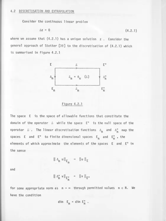
CHAPTER 4 GRADED MESHES
4.1 Rationale for Graded Meshes 4.2 Discretisation and Extrapolation 4.3 Shooting Methods .
I
4.4 First Order Case 4.5 Second Oroer Case - I 4.6 Second Order Case - II 4.7 Non-Optimal Choice of Mesh 4.8 Summary and Discussion
Appendix - Best Scaled Tridiagonal Matrices
CHAPTER 5 GRADED MESHES IN THE NAVIER-STOKES EQUATIONS 5.1 Solution Scheme for Graded Meshes
5.2 Choice of Graded Mesh 5.3 Discussion and Results
CHAPTER 6 SUMMARY 6.1 Summary
REFERENCES
Page 88 99 110 121 129 132
139 143 147
162
165
I
This work was carried out at the Computer Centre, the Australian National University. I gratefully acknowledge the financial assistance of a Commonwealth Postgraduate Award during this period.
I wish to thank my supervisor and the head of the centre, Mike Osborne, for the general support and encouragement that he has lent me and the constructive criticism that he has lent my work.
I wish to thank all the members of the centre for the welcome and friendliness that they have extended to me during my stay, and for the seminar, talks and discussions that they have contributed to my education.
I would also like to thank Lee Stirzaker for checking the manuscript for small errors and the typists Cheryl Riddell and
PREFACE
Part of the work in Chapter 4 in this thesis was done in collaboration with Mike Osborne especially that relating to first order formulations of the problem.
Chapter 2 in this thesis has been published as Woodford [46] and the text of that paper has been followed closely.
ABSTRACT
This thesis examines the use of graded meshes and extrapolation techniques in finite difference methods of solution for firstly, two-point boundary value problems and secondly, the prototype cavity problem. For equations of the form
d2v d
=---...t.... +a(x)* +b(x)y=O dx2
subject to the conditions
y(O) =y(l) = l ,
it is shown how to construct graded meshes that give optimum numerical properties to the finite difference scheme and also allow extrapolation processes, something that is not usually available when using graded meshes. Both first and second order formulations of the two-point
boundary value problem are examined.
Chapter 3 examines the cavity problem using a regular mesh while Chapter 5 uses graded meshes. Only the case of a Reynolds number of 50 is discussed for both divergence and convective forms of the vorticity transport equation. Extrapolation _is used in all cases. For the regular m_esh cases and one graded mesh cases, convergence is attained by the extrapolated results to within two significant digits. A mesh is
CHAPTER 1
THE PROTOTYPE CAVITY PROBLEM
1.1. INTRODUCTION
The prototype cavity problem concerns the fluid motion generated in a rectangular cavity by the uniform translation of the upper surface. The fluid in the cavity is viscous and incompressible. In this thesis, numerical solutions to the Navier-Stokes equations of fluid motion are sought to describe the fluid motion for middle range to high Reynolds
numbers where the Reynolds number is defined as Re= UL/v where U is the velocity of the upper surface, L the width of the cavity and v is
the kinematic viscosity.
The cavity problem is part of a larger class of problems of steady separated flows. This class of flows and in particular the cavity problem has been studied by Burggraf [8] both analytically and numerically. The fluid dynamic features of the cavity flows and of closely related flows
(e.g., with thermal effects added) have been extensively studied in the literature (Kawaguti [24], Mills [29],-Burggraf [8], Pan and Acrivos [33], Greenspan [22], Donovan D41, Torrance et al. [43], Runchal, Spalding and
Wolfshtein [38], Marshall and Van Spiegel [28], Bozeman and Dalton [5]). Experimental visualisations (Mills [29], Pan and Acrivos [33]) have been attempted but mainly for low to middle range (50 - 3,200) Reynolds numbers.
general aim of obtaining a solution for high Reynolds numbers. Though
questions may still be asked (see Bozeman and Dalton [5], Torrance [42]) about the finite-difference representations of the non-linear terms in the
Navier-Stokes equations, it is my feeling that the major finite-difference
approach via the use of evenly spaced grids has been fully extended and the problem of a solution for high Reynolds numbers is a matter of truely
excessive computer time. It is felt that finite differences using graded
meshes may provide an improvement in the solution of the problem. One of
the aims of this thesis is to explore the applicability of graded meshes as an alternative approach to the solution of the problem by difference methods.
The cavity problem has special interest as a prototype problem on
which to test numerical schemes. This special interest stems basically from the simplicity of formulation which implies a reduced complexity for the implementation of new numerical schemes and allows easy testing of the
many parameters in the models in the search for improvements in convergence,
1.2. FORMULATION OF THE CAVITY PROBLEM
Consider the cavity problem in terms of the physical variables. The Navier-Stokes equations for an incompressible fluid are
au
1 ....:::. + u·v'u = vv'2u - - v'p
at - - - p
and the incompressibility condition
where
v'•u = 0
uT = (u,v) is the velocity of a fluid particle,
v = kinematic viscosity, p = pressure,
p = mass density, t = time.
(1.2. la)
(1.2.lb)
Suppose the cavity with which we are dealing has width L , height D and the upper surface of the cavity is moving with uniform velocity U from
left to right. We define the non-dimensional variables
I
X = x/ L , I
y = y/L ' (u1
)T = (u/U, v/U) ,
p 1 = p/pU2 '
t1 = tU/L
a = D/L ( the aspect ratio) , Re = UL/v (the Reynolds number).
Substituting the variables into the equations (1.2.1), we obtain the equations (1.2.2) given below, the non-dimensional equations of fluid motion in a
a~
1 2-at + u•Vu = -Re Vu - - Vp (l.2.2a)
and
V•u = 0 ( 1. 2. 2b)
where the primes have been dropped from all variables because there can be no ambiguity as from this point, non-dimensional quantities are assumed. In equations (1.2.2), the boundary values are known only for the two velocity components, namely the velocity u = 0 at all walls except the upper surface where uT = (1,0). The boundary values for the pressure are
not known.
If the streamfunction-vorticity formulation of the equations (1.2.2) is used instead of the physical equations in the three unknowns (u, v and p), then only two unknown variables are sought, the stream function ~ and the vorticity w. The boundary values for this formulation are found naturally without the imposition of any extra conditions. Hence we consider the
stream-function-vorticity formulation of the cavity problem.
Eliminating the pressure variable p by taking the curl of equation (l.2.2a) ..,,,e obtain the vorticity transport equation in convective form
aw 1 2
- + u•Vw = - V w
at - Re (1.2.3)
where w represents the two-dimensional vorticity
av
au
w =
ax -
ay · (1.2.4)Using the condition (l.2.2b), equation (1.2.3) may be rewritten in divergence
form as
aw ( ) 1 2
We introduce a streamfunction ~ such that
and
u = ~
ay
V = - ~ ax·
( 1. 2. 6a)
( 1. 2. 6b)
From equations (1.2.6) we see that the incompressibility condition (l.2.2b)
is automatically satisfied. Substituting the equations (1.2.6) into the
definition of vorticity (1.2.4), we obtain a simple relationship between
the streamfunction and the vorticity
- 2
w - -'i/ ~ (1.2.7)
Since the boundary of the cavity is a stream-line, the streamfunction
is constant there. From the differential definition (1.2.6) of the
stream-function, its value is only determined to within an additive constant. We
set ~ = 0 on the boundary. This choice is helpful in some of the later
computation. All the boundary conditions for equations (1.2.3) and (1.2.7)
are available, namely the values of the streamfunction and of its normal
derivative at the boundary,
X
=
0, 0 < y < a, ~=
0,~=
ax 0 ,y
=
0, 0 < X < 1, ~=
0,~=
ay 0(1.2.8)
X
=
1, 0 < y < a, ~=
0,~=
ax 0Y
=
a, 0 < X < 1, ~=
0,~=
1.
ay
Because the derivatives of the streamfunction tangential to the walls
are all zero at the walls, the vorticity there is defined by a reduced form
w = (1.2.9)
1. 3. DESCRIPTION
The major flow in the cavity consists of a large primary eddy which
fills most of the square cavity and depending on the Reynolds number, there
may be two smaller and very much weaker counter-rotating eddies in the
lower corners. If the cavity is deeper then large secondary counter-rotating eddies may develop (see Pan and Acrivos [33]) in the lower
portions, again with smaller and weaker eddies in the lower corners.
For a square cavity (the only sort covered in this work) and a very low Reynolds number, the vortex centre of the large primary eddy is
located at about three-quarters of the cavity height and along the vertical
centre line of the cavity. A pair of smaller and very much weaker counter-rotating eddies develop in the lower corners of the cavity. As the Reynolds
number increases the vortex centre moves away from the centre line in the
direction of the local flow (left to right in this region) and down. With
further increases of the Reynolds number, the vortex centre moves further
down and towards the centre of the cavity.
As the Reynolds number increases and the vortex centre moves towards the centre of the cavity, the value of the vorticity across the central region of the cavity becomes approximately uniform. This behaviour is explained by Batchelor's [3] proposal that as the viscosity tends to zero
(or Reynolds number increases), the flow consists of a recirculating eddy
having uniform vorticity over an inviscid core with all the viscous effects being confined to small shear regions near the boundaries.
Batchelor's prediction of uniform viscosity in the central regions of the cavity for high Reynolds numbers is the major motivating force behind the
1.4. PREVIOUS INVESTIGATIONS
Burggraf [8] has completed an extensive numerical investigation
of the cavity problem. Using a modified relaxation method, he presents
results for Reynolds numbers of 0, 100 and 400 using an evenly spaced grid
in both directions with grid spacings of 1/10, 1/20, 1/30 and 1/40. His
solutions demonstrate the movement of the vortex centre of the primary eddy
towards the centre of the cavity as the Reynolds number increases and the
development of the secondary eddies in the lower corners of the cavity.
Burggraf notes that there is good agreement between the self-similar
solution for Stokes' flow in a corner as presented by Dean and Montagnon [13]
and modified by Moffatt [30] and the calculated result for the large corner
eddy at Re= 400. The secondary vortex pattern is completely viscous in
nature even though the primary eddy is relatively inviscid.
Pan and Acrivos [33] used the same relaxation technique as Burggraf
to obtain numerical solutions to the problem of creeping flow (Re= 0) in
a cavity of various aspect ratios. Numerical solutions were presented for
cavities with aspect ratios of 0.25, 0.5, 1, 2, and 5 using mesh sizes from
0.01 to 0.025. These solutions and those of Burggraf complement the
earlier results of Kawaguti [24] for aspect ratios of 0.5, 1 and 2.
Unfortunately Kawaguti 's results are somewhat inaccurate because of the
rather coarse (1/10) mesh size used. In Kawaguti 's work, the primary vortex
centre moved downstream towards the wall as the Reynolds number increased and
secondary eddies did not develop in the lower corners.
Pan and Acrivos found the primary vortex to be symmetrical for all
cavity depths considered. In the corners they found a sequence of
counter-rotating eddies of decreasing vortex strength and size. Moffatt's work was
solution had been obtained for the primary flow. Because of numerical
instability problems encountered by Burggraf for Reynolds numbers greater
than 400, Pan ~nd Acrivos did not extend their numerical experiments past
the creeping flow problem.
Reported in the same paper are flow visualisation studies attempted
by Pan and Acrivos for cavity flow over a wide range of Reynolds numbers.
For a square cavity the Reynolds number attempted ranged from 80 to 4,000,
the upper limit being the point at which flow instability began to appear.
The experiments produced flows that are consistent with Batchelor's
proposals. The numerical results available agreed with the flow visualisation
studies carried out for the parameters involved.
Mills [29] is reported to have examined the cavity problem both
numerically and experimentally for a Reynolds number of 100 and aspect
ratios of 0.5, 1 and 2. Full copies of his work were not able to be obtained
by this author though Donovan [14]includes some of Mills' flow visualisations
in his paper. His work is also mentioned in Burggraf [8] and the reference
is included for completeness.
Greenspan [22] considers the cavity problem numerically using a
generalized Newton's method with over-relaxation. He obtained solutions
for Reynolds numbers of 200, 500, 2,000 and 15,000 using a mesh spacing of
1/20 and for Reynolds number of 50, 104 and 105 using a mesh spacing of 1/40.
Secondary eddies in the lower corners were not found for the calculations
performed using the mesh size 1/20 for any Reynolds numbers yet other authors
(Pan and Acrivos [J3], Bozeman and Dalton [ 5] ) have found such eddies. In
Dorr[l6], a one-dimensional analogue of the Navier-Stokes equations is
representations of this analogue. Dorr found that the resultant algebraic
equations could become badly ill-conditioned if care were not taken. He
demonstrates an example that shows one cannot always determine whether an
iterative method has converged by simply looking at the difference between
successive iterates. This convergence criterion is used by Greenspan and
is not felt to be adequate for accurate solutions of the cavity problem by
his method.
Donovan [l4]solves the time dependent physical equations rather than
using the usual streamfunction-vorticity formulation. He uses a combination
of an explicit time stepping method and an over-relaxation technique to
solve the coupled equations for pressure and velocity. Solutions were
obtained using a mesh width of 1/20 for a Reynolds number of 100 and aspect
ratios of 0.5, 1 and 2. For a square cavity he also obtains solutions for
Reynolds numbers varying from 100 to 500. The solutions demonstrate the
movement of the vortex centre of the primary eddy towards the centre of the
cavity as described by Burggraf but there is no indication of the development
of secondary eddies in the lower corners for any Reynolds numbers.
Marshall and Van Spiegel [28] attack the streamfunction-vorticity
formulation of the problem by perturbing the streamfunction equation into a
time dependent equation where the time derivative of the streamfunction is
multiplied by a small positive parameter. The vorticity equation and the
perturbed equation are solved explicitly on an even spatial grid of mesh
width 1/10 for Reynolds numbers between 0 and 200 and mesh widths 1/20
and 1/40 for a Reynolds number of 400. Excessive computing time made
solution of the equations impractical for Reynolds numbers greater than 400.
The development of the flow is close to that of Burggraf but the development
lower Reynolds numbers possibly because of the coarse mesh size.
Bozeman and Dalton [5] have compared the effects of different
methods of differencing the vorticity equation written in either divergence
or convective form. The two methods of differencing the non-linear terms
(V•(wu) and u•Vw respectively) in either form of the equation were
central differences using second order correct difference quotients and
unidirectional differences using first order correct difference quotients
which are backwards with respect to the local direction of flow. The
boundary values of the vorticity were calculated using a third order
correct formula in preference to the usual first or second order correct
formulas. The equations were solved by the strongly implicit procedure
(SIP) of Stone [40).
The central difference, divergence form of the equation demonstrated
clear superiority for a Reynolds number of 100 and mesh sizes between 1/20
and 1/50. Both central difference formulas failed to satisfy the convergence
criterion (residual less than a specified value) for Re= 1,000 while
both unidirection forms did.
The solution obtained with unidirectional differences and divergence
form is consistent with Batchelor's model and similar to previous flows
reported while that in convective form was inconsistent with the expected
flow, there being two large vorticies instead of one occupying the cavity.
The superiority of the divergence form is also mentioned in Torrance et al.
[43). Convergence was not obtained for Reynolds numbers greater than
1,000 for any method.
u
convection added. Thermal boundary conditions treated have been, after non-dimensionalizing, (A) zero on all walls except the moving upper
surface where the temperature is unity, and (B) zero on the bottom, unity on the top with a continuous linear variation along the side walls.
Condition (B) was considered by Runchal, Spalding and Wolfshtein [38]. The equations were written in a finite difference form involving unidirectional derivatives that led to conservation of momentum and energy over the grid and to positive definite equations. These equations were solved by
relaxation techniques on a 13 x 13 non-uniform grid for Reynolds numbers
3
of 1 and 10 . Unfortunately the method for choosing the graded mesh was not explained and general rules were not proposed. The results agree quite well with earlier work and with Batchelor's model for large Reynolds
numbers.
Torrance et al. [43] examine the combined effects of a moving wall and natural convection via case (A) for aspect ratios of 0.5, 1 and 2 and for Reynolds numbers of 100, a Prandt'l number of 1 and for various Grashof numbers including zero. The equations were written in divergence form. Forward time and central space differences were used for all terms except the convection terms for which special three point non-central differences were employed. Explicit time stepping is used to solve the time dependent equations but only the steady state solutions are presented. The Poisson
equation for the stream function is solved by over-relaxation. A mesh spacing of 0.05 is used for an aspect ratio of unity. Velocity profiles and streamfunction values are in close agreement with Donovan [14] and in fair agreement with the works of Mills [29] and Kawaguti [2~ who used comparatively coarser mesh spacings. It is suggested that a mesh interval of 0.05 by Torrance et al yields results comparable to a mesh spacing of
results is the use of a finite difference representation of the
convection term (written in divergence form V•(wu)) that conserves
vorticity within the grid. Vorticity patterns were not presented and
could not be compared.
For completeness and also to give an example of a possible
application of this work, Frommrl9]considers case (B) but without a moving
upper surface. He considers the time dependent vorticity and energy
equations with the Boussinesq approximation. These equations are
differenced to fourth order accuracy and solved explicitly. The Poisson equation for the stream function is solved by the Buneman direct method
(see the review by Dorr [15]) over a 65 x 65 grid. Batchelor's model as
discussed in Burggraf [~ implies the temperature will be uniform to first order in a closed cavity even for a non-circular eddy. Fromm's solutions
for a range of Grashof and Prandtl numbers bear out this result.
Chorin [9] has examined the convergence of discrete approximations
to the Navier-Stokes equations. Besides excluding turbulence from the
range of application of difference methods (see Chorin[lO]) his discussion
in [ g] suggests that there is no good reason for always casting the
non-linear terms of the Navier-Stokes equations in "conservation form", i.e. in
a form which implies the existence of identities for the momentum similar in appearance to those which hold for the solutions of the differential
equations. Chorin in fact has not endeavoured to do so but approximates
-CHAPTER 2
DIRECT SOLUTION OF THE POISSON EQUATION
2.1. INTRODUCTION
The streamfunction-vorticity relationship takes the form of a
Poisson equation with Dirichlet boundary conditions,
2
V l/1 = -w
and 1/J = 0 on the boundary
(2.1.1)
In the iteration scheme to solve the two coupled equations describing the
cavity problem flow, equation (2.1.1) needs to be solved for l/1 given
the values of w inside the rectangle. Details of the complete numerical
scheme are given in Chapter 3. In this scheme equation (2.1.1) is solved
repeatedly; considerations of efficiency in its numerical solution become
of paramount importance.
Consider Poisson's equation on an N x N evenly spaced grid over
the unit square. The relative computing costs of several different methods
are displaced in Table 2.1.1. In this table and in the ensuing work, one
computer operation is defined to be a floating-point multiply and add.
Some of the estimates used there can be found in [271. The computational
costs of two iterative methods are displaced in Table 2.1.1. The operation
counts for these methods have been calculated for asymptotic rates of
convergence to the same relative accuracy as the difference equation
approximates the differential equation. It is assumed that optimal
TABLE 2 .1.1
Operation counts for the solution of Poisson's equation on a rectangle. Method of Solution
Optimal Successive Over-relaxation
Bickley-McNamee [4]} (PP) Tensor Product [27]
Alternating Direction Implicit
Direct Method (PP)
Direct method using Winograd's algorithm for a UNIVAC 1108
computer. (PP)
Direct method using conventional FFT*
Direct method using new FFT*
Operation Count
3
14N log10 N
40N2 1 oglO 2 N
(PP) This method has a pre-processing overhead not shown in the operation count (see text).
* FFT = Fast Fourier Transform.
From Table 2.1.1,it is obvious that the algorithms using the FFT are
significantly more efficient than other methods. However, in this work we are specially concerned with graded meshes and the special forms that allow the FFT algorithm to be used depend critically on the formalism of the
problem when an even grid is used. If a graded mesh is used in this problem
then the direct method suggested in this work, including the use of Winograd's
[image:22.611.64.596.13.769.2]A detailed explanation of the notation and the structure of the
finite difference scheme used is given in §2.2. In §2.3 a formal analytic
solution of the Poisson equation is derived and it is then shown that
this formal solution has a computationally advantageous counterpart in
the finite difference formulation. For an even mesh the special advantages
gained by the use of Fast Fourier Transform are demonstrated in §2.4 while
in §2.5, Winograd's method for matrix multiplication is examined for
efficiency. This method is advantageous in the multiplication of medium
size full matrices and such matrices are of special concern in the cavity
2.2. NOTATION FOR THE POISSON EQUATION
The problem considered here is slightly more general than the
streamfunction-vorticity equation with its zero boundary conditions.
Without loss of any generality we restrict attention to a square region
and consider the Poisson equation
;/u 2
-2 (x,y) +a~ (x,y) = f(x,y)
ax ay (2.2.1)
for (x,y) € R = (0,1) x (0,1) with the Dirichlet boundary conditions
u(x,y) = g(x,y)
for (x,y)E aR.
Consider a mesh where the lines parallel to the y-axis have
abscissae
and the lines parallel to the x-axis have ordinates
(2.2.2)
(2.2.3)
The following method does not require evenly spaced grid lines but
for simplicity of presentation, we con_sider only an evenly spaced grid in
this chapter. Where differences would arise because of unequally spaced
grid lines, those differences will be noted in the text.
Let h and k be the spacings between the grid lines in the x and
Y directions respectively. If the value of a function u(x,y) at the mesh
point (x.,x.)
l J
for appropriate
is represented by the element u .. = u(x.,y.) of a matrix l J l l
the interior of the unit square are in the matrix
U = [U , U , ••• , U ] , - 1 -2 -m
where
uJ'. = ( u 1 . , u
2 . , ••• , u . )
- J J nJ
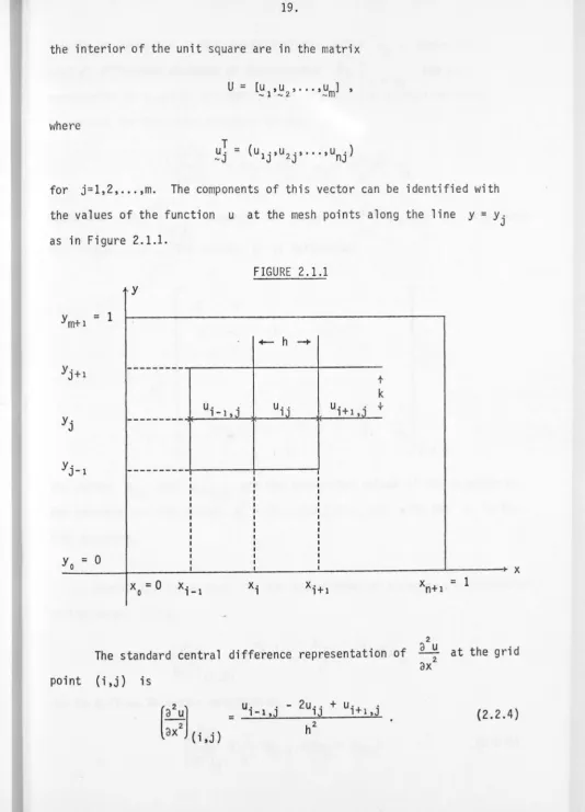
for j=l,2, ... ,m. The components of this vector can be identified with
the values of the function u at the mesh points along the line y = yj
as in Figure 2.1.1.
Y·
J [image:25.617.66.600.14.755.2]= 1
FIGURE 2.1.1
y
+- h
--+-
---,---+----+---t kU i -l , j U i j U i + 1 , .i f
---~__:._;:_.,_,,_-l!E----'-'='----,lf-_;_--'-"--
---1---+---y = 0
_:_o _ _ _ -+-_ _ _ _..:.. _ _ _ _ .:..._ _ _ _ _,_ _ _ _ _ _ _ _ _ ..__ _ _ _ X
X = 0
0
x.
1-1 X, 1= 1
2
The standard central difference representation of
.£..J!.
at the gridax
2point (i,j) is
[
a
2
u]
ax
2 ( • • )l ,J
= ui-i,j - 2uij + ui+i,j
This is an operation on the elements of the vector uJ . . Hence the
2
-central difference analogue of the operator
~
I
can beax Y = Y ·
represented by a matrix pre-multiplication with some colrection terms
to account for the known boundary values:
[:)t
= Au.-J
where the vector
["';]
contains ax .J
for i = 1 , 2 , ... , n The matrix A
--2 1
- 1
A -h2
1 -2
u . u .
+ ~ e1 + n+1 ,J ~n
h2 h2
2
the values of a ~ ( Xi ,y j ) as ax
is defined by
-1
1 -2 1
1 -2
- n x n
components
The values u
0J. and u n+1 ,j are the prescribed values of the solution on T
the boundary and the vector e.
_,
= (0, ... ,0,1,0, ... ,0) with the 1 in thei I th position.
Similarly, the formula for the calculation of a second y - derivative
at the point (i,j),
(
a
2
u]
a/ (
1..
,J)
Ui,J.-l - 2u .. + u. ·+
= lJ 1 ,J l
k2
can be written in vector notation as
= J_ ( u. - 2u. + u ·+ ) k 2 -J - l -J -J l
[
;/u]
where the vector
-ay2
j2
-
a
ucontains the values of - (x.,y.) for
a/
,
Ji=l,2, ... ,n . For j = 1 and j = m, the prescribed boundary values
~o and ~m+l are used in equation (2.2.5).
The discretised Poisson equation can be written as
1 I
Au.+ - (u. - 2u. + u.+) = f.
-J k2 -J-1 -J -J 1 -J (2.2.6)
for j=2,3, ... ,m-1 , where
I 1 1
f . = f . - - u .e - - u .e -J -J h2 o,J -1 h2 n+1,J -n
where u .
o,J and u n+1 ,J . are the known values of the solution on the
boundary. For j = 1 and j = m, the known boundary values ~0 and
um+ must be taken into account. Hence for j = 1 , the equation (2.2.6)
- l
becomes
where
f' = -1
and similarly for j = m
Au + _l_ (-2u + u) = f1
-1 k2 -1 -2 -1
u Un+ 1, 1
f - - e 0 l ~n
--1 h2 - l h2
.
-1..u k2 -o
In equation (2.2.6) linear combinations of column vectors from
the matrix U are used in the calculation of the second y-derivative. The
above notation allows this operation to be written as a matrix
post-multiplication. Thus the equations (2.2.6) for j=l,2, ... ,m may be written
as
-
--2 1
1 -2 .
AU+ U·p 1 1 = F' {2.2.7)
1
-2
-where
F1
f1 f1
I
= [ 1' 2, . . . , f ] •
- - -m
Without ambiguity, the primes may be dropped from the fi and the F1
in equation (2.2.7). Defining the matrix B as
--2
1
1
-2.
1
-1
-2
- m x m
the discretised Poisson equation with Dirichlet boundary conditions on the
given grid becomes
AU + UB = F • (2.2.8)
Note that both of the matrices A and B are symmetric and
tridiagonal. In fact for an evenly spaced grid in the x(y) direction,
the matrix A(B) has a constant diagonal and constant and equal sub- and
super-diagonals. The special properties that follm-.i from this situation
are discussed in §2.4. For a more general graded mesh, the weights in the
three term relationship used to calculate the second derivatives change
from the simple ( 1 _:_g_
...L]
to a more complicated and unsymmetric~ , h2 , h2
pattern.
If we have the mesh (2.2.2) and (2.2.3) and we define
i=0,1,2, ... ,n
then the second x-derivative can be approximated at the (i,j) mesh point
- :,
[
a
2u]
ax
2 ( • • )l ,J
2u. . = l+l,J
h.(h. + h. ) l l l - 1
2u .. lJ h.h.
l l - 1
2u. . + l - 1 ,J
h. (h.+h.)
1-1 l 1-1
(2.2.9)
An equivalent expression is used for the second y-derivative. Note that in the central difference formulas (2.2.4) and (2.2.5) for the calculation of a second derivative on an even mesh, the discretisation error is O(h2
).
For a graded mesh, the accuracy with which the difference equations
approximate the differential equation is degraded to first order. At the (i,j) mesh point, the formula (2.2.9) approximates a second derivative with a minimum discretisation error of O(h.-h.
1) + O(h1. 2+h.2
1). When expanded
l ,-
,-about the central point by a Taylor series expansion, any other central three point formulas have a larger discretisation error.
With graded meshes even if formulas with minimum discretisation error are used in the approximation of the differential equations, there is an overall loss of accuracy in the approximation of the continuous problem by the difference equations compared with the use of central
difference formulae on an equivalent even mesh. This loss of accuracy must be reflected in the solution of this problem. In §4.1, an example is given where a well behaved equation is solved on an even mesh and on a randomly chosen graded mesh. A comparison of these two solutions with the analytic solution clearly demonstrates the effects of careless use of graded meshes.
If a systematic scheme can be found for choosing the mesh points of
a graded mesh, then mesh refinement becomes a simple task and extrapolation procedures may possibly be brought into action to improve the accuracy. For
- ,!
differences on an evenly spaced mesh with a large number of points. For
discussion of such problems and for the suggestion of one such technique
see Chapter 4.
When graded meshes are used in the solution of Poisson's equation
on a rectangle, then central three-point formulas like formula (2.2.9) have
the advantage that the resulting matrices A and Bin equation (2.2.8) have
their tridiagonal form preserved. In general though the symmetry and the constancy of the three diagonals will be lost, resulting in serious
consequences for the computational efficiency with which the problem may be
2.3. DIRECT SOLUTION OF THE POISSON EQUATION
Pre-multiplication of the solution matrix U by the matrix A is
2
equivalent to the application of the operator L =
_a_
to the functionx
ax2
u(x,y). Similarly, post-multiplication of the matrix U by the matrix B is equivalent to the
function u(x,y). With
2
application of the operator L = ~ to the
Y ay
these correspondences in mind, let us examine one
method of solution for each of equations (2.2.1) and (2.2.8).
are the eigenfunctions and
eigen-values of the operator LY, that is ,
The functions u(·,y) and f(· ,y) can be expanded in the eigensystem as
CX)
(2.3.la)
and
CX)
for appropriate coefficients uk(x) and fk(x) . Substituting the equations (2.3.1) into equation (2.2.1), we obtain
Lx u(x,y) + LY u(x,y) CX)
=
l
{(Lx + Ak) uk(x)} ¢k(y)k= 1 CX)
(2.3.2)
These equations can be solved by any suitable method, then knowing the
solution functions {uk(x)};=i , equation (2.3.la) may be used to reform
the solution u(x,y) . Note that the eigenfunctions of the operator
a2
L = - are sines in this case; this will be important in §2.4 in the
Y
ay2discussion of the use of the Fast Fourier Transform.
Consider now the finite difference equivalent of the above scheme.
The eigensystem of the matrix B is
(2.3.3)
where the matrix Q is orthogonal, that is QQT = I and QT means the
transpose of Q. Let Q be partitioned into column vectors as
where q'. = (q .,q ., ... ,q _, 11 21 nn .) for i=l,2, ... ,m. If equation (2.3.3) is
substituted into equation (2.2.8), then we have
AU + UQ AQT = F
Post-multiply this equation by the matrix Q and defining
lJ = UQ (2.3.4a)
and
f'" = FQ , (2.3.4b)
we obtain
AU+
U
=f.
(2.3.5)Note that equation (2.3.4) is the finite difference equivalent of finding the coefficients uk(x) and fk(x) from the formula
1
uk(x) =
f
u(x,y) ¢k(y) dyfor the continuous case. Compare this with the expansion of equation (2.3.4a) as
m
=
l
UiJ. qJ. kj=l
where the uik are the coefficients of the eigenvectors q. in the
-J expansion of U
Take the j'th column of equation (2.3.5) to obtain the separated equations
(A + ". I)u. =
f.
J -J -J (2.3.6)
for j=l,2, ... ,m. Each equation of (2.3.6) is the finite difference
equivalent of an ordinary differential equation in x for the transformed
functions uk Each is a simple symmetric tridiagonal linear system of equations in n variables. Using simple Gaussian elimination on the tridiagonal system requires Sn operations for its solution. These are m systems in equation (2.3.6) hence a total of 5nm operations are
necessary to solve for the matrix IT. Then from equation (2.3.4a) we find
u
=UQT.
This matrix multiplication takes nm2 operations as does the multiplication
in equation (2.3.4b). These two matrix multiplications and the solutions of equations {2.3.6) make a total of
2nm2
+ 5nm operations
for finding the eigensystem of B is considered a preprocessing overhead. Note that for an evenly spaced y-mesh the FFT algorithm can be used as explained in §2.4, and the eigensystem of B is never explicitly found so that this preprocessing overhead does not exist in that case.
The method of solution of equation (2.2.1) using an evenly spaced
mesh in at least one direction as discussed above is not adequate if unequally spaced meshes are used in both directions. In this case the finite difference equations arising from equation (2.2.1) has a matrix B which is still tridiagonal but is not now symmetric. The previous method of solution hinged on the fact that the left and right eigenvectors of B were identical. This is a consequence of the symmetry of the matrix B For unsymmetric B with positive off-diagonal elements, there exists a
diagonal similarity transformation that changes B to a symmetric tridiagonal
matrix S, namely
where D is a diagonal matrix.
If we substitute this into equation (2.2.8), then after post-multiplying by the diagonal matrix D, we have the equation
AUD+ UDS =FD.
By defining U
1 = UD and F1 =FD, this last equation becomes
The matrix S is symmetric so this equation has the same form as equation (2.2.8). Hence the previous method of solution can be used to solve for
U1 from which U is found by the diagonal matrix multiplications
multiplications for the two diagonal matrix multiplications. This makes the total operation count only slightly larger. In fact, it is dwarfed by the major cost of the solution - the 2nm2 operations for
the two full matrix multiplications.
2.4.
USE OF THE FAST FOURIER T
RANSFORM
For a mesh with equally spaced grid lines in they-direction, the
matrix B in the discretised Poisson equation
(2.
2.8
)
has the form-
--2 1
1 -2 .
1
1
l -2
-- - m x m
The eigenvalues of this matrix B are
and the eigenvectors q. have components
-J
j=l,2, ... ,m
i. i=l,2, ... ,m q . . = C S i n...21..'!!_
1J m + 1 ' J=l,2, ... . ,m
(2.4.1)
where c is a common normalising factor. For the method of solution
introduced in §2.3, let us examine one of the matrix multiplications FQ
or UQ T , say
r
= FQ For one element ofF
we havem
t ..
=2
f H q.e.J· lJ R,=l= c
I
fH sinm.e,i\ .R,=l
(2.4.2)
*
Let the rows of the matrix F be the vectors
!;
so that*
f. = (f. ,f. , ... ,f. ) , i=l,2, ... ,n .
-If these row vectors are considered as vectors of data, then equation
(2.4.2) is just a discrete sine transform of that data. This should not 2
be surprising since the eigenfunctions of the operator ~ are sines
ay
in this case and we are here discussing the finite difference equivalent
of that operator, the matrix B.
A discrete sine transform can be performed very quickly just by
*
taking the FFT of the f. as real data and taking the imaginary
_,
component of the complex result or, as explained in [11], the FFT algorithm
[12] can be used to perform just a sine transform on real data for little
extra work. Hence the matrix multiplications FQ and UQT can each be
performed for a computational cost of
2nm log
2m operations
This is a distinct reduction from the nm2 operations needed for those
matrix multiplications by the usual inner product method. There is the
added bonus in the solution of the Poisson equation of no preprocessing
overhead to find the eigensystem Q and A of the matrix B as there is
in the method in §2.3.
With an even grid in the y-direction, the Poisson equation over a
square region with Dirichlet boundary conditions can be solved in
4nm log m + 5nm operations .
2
There are reports [21] of a new stable method for the FFT algorithm
that takes O(m log
2(log2m)) operations for m data points. The use of
this new algorithm instead of the usual FFT algorithm (O(m log2m) operations
for m data points) would decrease the above operation count even further.
the theoretical lower limit for the FFT algorithm is O(m) operations
which would imply O(nm) operations for the Poisson equation. Methods
which achieve this are not currently known.
For the Poisson equation as above but also with an even grid in
the x-direction, the matrix A also has the form of (2.4.1). Hence for
solving the set of equations
(A+ A,l)u.
,
_,
=f.
_,
i=l,2, ... ,m;the same use may be made of the FFT algorithm. Because the FFT algorithm
takes O(n log
2n) for these equations and simple Gaussian elimination takes O(n) , the use of the FFT algorithm in this case is not recommended.
The FFT algorithm is not limited only to the Poisson equation. The
method described in §2.3 may be applied to any second order linear
separable elliptic operator and the FFT algorithm may be used to perform
the appropriate matrix multiplications if the resultant matrix B has the
2
form of (2.4.1). This will occur for example if the operator L =_a_+ c
Y
a/
2.5. WINOGRAD's METHOD OF MATRIX MULTIPLICATION
Since the major computational cost in the solution of equation (2.2.1) is in the matrix multiplications FQ and UQT, a more efficient method of matrix multiplication than the usual inner product method would be welcome. We will demonstrate an algorithm for matrix multiplication which uses Winograd's identity [45] for an inner product. This algorithm performs the multiplication of two n x n matrices in less than n operations.
For n even (extend the vectors to length n + 1 by adding a
zero as the last component if n is odd), Winograd's identity for the inner
product of two n vectors
and
n/2 a=
.l
J=l and
X • • X . 2J 2J - l
are known, then Winograd's identity is
is: if
On the left of this identity is the no_rmal inner product formula which requires n multiplications and n - 1 additions (we make no distinction between addition and subtraction). On the right of the identity is
Winograd's form of the inner product. This requires
i
multiplications and~
+ 1 additions. In Winograd's formula, half(2"]
of themultiplications are exchanged for slightly more than half·
(¥-
+2)
additions.whatever data types being used, that is, single or double precision, real
or complex numbers.
For the matrix multiplication Z = XY say, of two n x n matrices
X
andY,
we compute a number ai for each row of the matrixX
and anumber Sj for each column of the matrix
Y
at a computational cost of2"
multiplications and ~ - 1 additions for each of these 2n numbers. We
then use these numbers in the computation of the n2 inner products needed
to form the matrix
Z,
for
and
and
n/2
z .. =
I
(x. k + y k .)(x. k + y k .) - (a. + s.)l J k= 1 l , 2 2 - l , J l , 2 - l 2 , J l J
i=l,2, ... ,n and j=l,2, ... ,m. This method
3
lQ_ + 2n(n - 1) additions compared with the 2
3 2
additions. n - n
If on a certain computer
f = time for multiply
time for add
takes 2 n 3 + n 2 multiplications
usual n3 multiplications
since an operation is one multiply plus one add then one operation is f + 1
adds. If W is the computational cost of an n x n matrix multiplication
using Winograd's identity and if IP is that computational cost with the
usual inner product, then neglecting terms of order n for simplicity, we
have
and
[n
3 2] +(3~
3
+
2
n
2J
W = f y + n _
f + 1
fn 3 + n 3 - n 2
Ip = ---::---:---f + 1
Both W and IP are in units of operations. The condition for some savings
w
w
< 1For a given f this condition is satisfied if the order of the matrices satisfies
n > 2 f..±....l f - 1 .
If we let W/IP = R the relative efficiency of the two methods, then Figure
2. 5 .1 presents a graph of relative efficiency versus order of the matrices for various values of the machine constant f.
For a Univac 1108 computer with f = 1.625 for single precision floating point arithmetic, we find that n must be greater than 14 for
some saving to be made. For larger n on a Univac 1108, the cost for Winograd's method is
3 2
W = 0.881n + 1.381n compared with the inner product method's cost of
IP= n3
- 0.38ln2 •
Hence the break-even point for the use of Winograd's method is just raised
slightly.
One application of Winograd's method is in the iterative use of
equation (2.2.1) since each time the equation is solved, there are two
matrix multiplications to perform. Assuming that for an n x n system,
the size n is large enough to satisfy the requirements of Winograd's
algorithm on the computer being used, then some small but significant
saving may be had. For example, on a Univac 1108 the cost of solving
equation (2.2.1) reduced to
3 2
1.77n + O(n) operations
compared with the usual
2n3
+ O(n 2) operations.
Another method for the efficient multiplication of very large full
matrices is that of Strassen [41]. The computations for the multiplication of 2 x 2 matrices are rearranged to .take 7 (usually 8) multiplications and
18 (usually 4) additions. This rearrangement does not depend on the commutativity of the objects being multiplied (as does Winograd's method) and so may be applied recursively to block matrices of size 2k to perform matrix multiplication in O(n10g27 ) ~ O(n 2'8) operations. Strassen's method
with one depth of recursion is faster than the normal method for n ~ 100 or higher depending on the machine. Significant gains of 7% to 13% are realised
by Winograd's method for matrices of this order so that Strassen's method which is much more difficult to code only becomes advantageous for much larger matrices.
Brent [7
J
discusses efficient methods for matrix multiplication and for anIBM 360/67, his formulas suggest that Strassen's method with one depth of recursion overtakes Winograd's method for real arithmetic at about
r..: t")
" -Q_ 1---l ..._m3:
.
' - / ~>-UCO
z
w·
1---l ~u
1---l
LL
r----LL •
w~
w
> 1---l (DI- •
o:~
_J
w
0:::LD
.
~0
20
40
_ _ _ _ _ _ _ _ _ _ _ _ _ _ _ _ _
LF
1
.50
_ _ _ _ _ _ _ _ _ _ _ _ _ _ _ _ _ _ _ _ _
LF
1.75
_ _ _ _ _ _ _ _ _ _ _ _ _ _ _ _ _ _ _
____[F 2.00
_ _ _ _ _ _ _ _ _ _ _ _ _ _ _ _ _ _ _ _ _ _LF
2.50
_ _ _ _ _ _ _ _ _ _ _ _ _ _ _ _ _ _
LF
3.00
_ _ _ _ _ _ _ _ _ _ _ _ _ _ _ _ _ _ _
_c__:F 5. 00
- - - . ! . . . : F - 1 0 . 0
60
80
SIZE
OF MATRICES
100
120
140
160
180
200
Figure 2.5.1 Graphs of the theoretical relative efficiency (W/IP) of Winograd's
algorithm for matrix multiplication to the usual inner product method versus the size (n) of the matrices for various values of
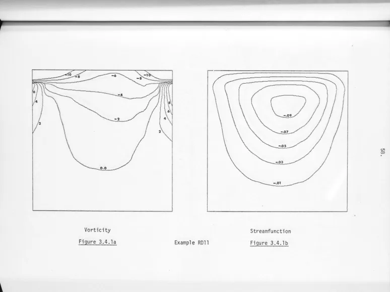
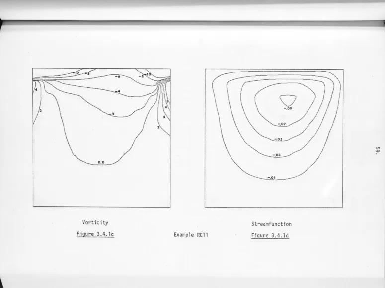
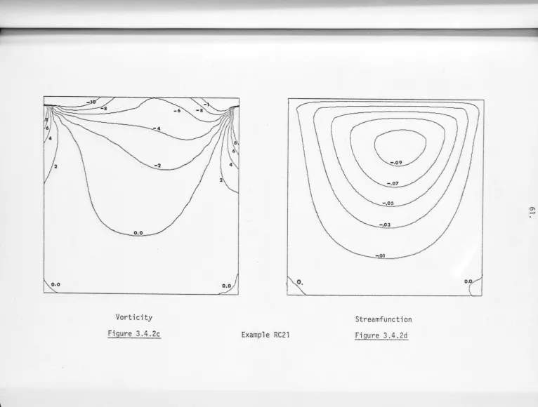
[image:43.788.32.777.18.566.2]CHAPTER 3
THE NAVIER-STOKES EQUATIONS
3.1. THE SPACE DERIVATIVES IN THE VORTICITY EQUATION
Consider the vorticity transport equation in divergence form
aw + ..l_ (wu) + ..l_ (wv) = 1 "i/2
at ax ay Re w (3.1.1)
where
u = ~ and v = - ~
ay ax (3.1.2)
The physical boundary conditions for this equation are no slip and no
penetration conditions on the walls of the cavity and are given in (1.2.8).
For the discretisation of the space derivatives in equation (3.1.1), we use
the graded mesh
0 = = 1
and
0 = y o < y < y < ••. < y < y = a .
1 2 m m+1
Let hi= xi+i - xi for i=O,l, ... ,n and kj = Yj+i - yj for j=O,l, ... ,m.
Appropriate linear combinations of the function values at three adjacent mesh
points are used to approximate the values of the space derivatives in
(3.1.1) at the central mesh point of the triple. With an evenly spaced mesh
central difference schemes would be sufficient to ensure second order
discretisation error but we are mainly concerned with graded meshes which
The first term approximated from equation (3.1.1) is the difference
term V2w. From equation (2.2.9) the three point approximation formula
for a second derivative over a general graded mesh leads to the formula
2
(V w) . .
l ,J
2w. . 2w . .
= 1+1,J l,J
h.(h.+h. )-h.h.
l l 1-1 l 1-1
2w. .
+ 1-1,J
h. (h.+h. )
1-1 l 1-1
2w. . 2w ..
+ l 'J + l l,J
k.(k.+k. )-k.k. J J J-1 J J-1
2w . .
+ l ,J -1
k. (k.+k.)
J-1 J J-1
(3.1.3)
The discretisation error for this formula is minimum in the sense that, for a general function that has fourth order continuous derivatives over a general graded mesh, any other pair of three point formulas
approximate second derivatives to a lower order of accuracy. For the above
formula (3.1.3), the discretisation error is O(h.-h. )+O(k. -k. ).
l 1-1 J J-1
If the mesh is equispaced in both directions, the above formula reduces to
the standard five point approximation to the Laplacian
(V2w). . = l ,J
w. . - 2w . . + w. .
1-1,J l,J 1+1,J
h2
+ wi,j-1 - 2wi,j + wi,j+1
k2 (3.1.4)
which has discretisation error O(h2) + O(k2) where h and k are the mesh spacings in the x and y directions respectively.
At points of the mesh for which
=
1 or n or j=
1 or m ,the values of the vorticity on the boundary are needed in the calculation of the diffusion term. The boundary values for the problem do not include the
vorticity on the boundary but the wall vorticity can be approximated
normal velocity component. From equation (1.2.9) the vorticity at the
walls is expressed by
w = -
~
an
2 (3.1.5)where n is the normal to the wall. Suppose the streamfunction values are known at all mesh points. The first normal derivative of the streamfunction ~
a
n
is known at the walls from the no slip condition. The wall vorticity(3.1.5) can be approximated by a three point relation with second order
discretisation error
where the subscripts denote function values at different mesh lines away from the wall, 0 being the wall line, and where
a
= -
(8 + y)'
8
2(h0 + h1)
-
-
2ho h1
(3.1.6) 2h0
y
=
2 '
(ho + hl) hl
-2(2h + h )
0
=
0 1(ho+ h1)ho
where h0 is the distance of the first mesh line from the wall and h1 is the distance of the second mesh line from the first.
The streamfunction is determined only to within an additive constant
w O = 8 iJJ l + y iJJ 2 + cS ( ~ ] 0 •
From the boundary conditions (1.2.8), the normal derivative of the
stream-function at the boundary is zero except for y = 1 where ~ = 1 . The
wall vorticity calculations simplify to
WO ,j = 8 iJJ l ,j + y iJJ 2,J .
w . = 8 1/Jn,j +yiJ;n-1,j + cS n+ 1, J
for j=l,2, ... ,m
'
and (3.1.7)w. = 8 iJJ i , 1 + y iJJ.
1 , O 1 , 2 '
w. 1 ,m+ 1 = 8 iJJi,m + Y iJJi,m-1 for i=l,2, ... ,n
'
for appropriate S's , y's and cS as given in the equations (3.1.6). The
formulas (3.1.7) have second order discretisation error. This error is either
the same order as or higher order than the approximation of vorticity in the interior of the cavity. So approximations to the boundary values do not
degrade the accuracy of the approximations in the interior.
For the special case of an even mesh in both directions, the equations (3.1.5) simplify to
8 = 4 k2
1 y = -2
2k
cS =
-
-
3'
k2
formulas hold for the walls x
=
0 and x=
1 .Consider the convection term in divergence form
( )
_
a
a
V• w
-
u - -ax
(wu) + -a
y
(wv)·
The velocity components are obtained by numerical differentiation of the
streamfunction then the products wu and wv are differentiated
numerically and added to obtain the final value. In the calculation of a
first derivative, a three point formula is used to approximate the derivative
value at the central point. The coefficients in this formula are chosen so
that if the terms are expanded about the central point by a Taylor series
expansion, then as many as possible lower order contributions to the error
cancel. For example, the first x-derivative of the streamfunction is
calculated from the formula
h.
l - 1
= h.(h. + h. } • 1/1;+1,j +
l l l - 1
(h. - h. )
l l - 1 h. h.
l l - 1
• 1/1 • • 1 ,J
h.
l
h. (h. + h. } • ljii-1,j
1-1 1 1-1
(3.1.8)
The discretisation error for this approximation is 0 ( h · h 1 l -· 1 ) , a first
order error. Similar expressions hold for first derivatives with respect to
y . Where even meshes are used, equation (3.1.8) reduces to the usual two
point central difference approximation
(~'-
tJ
. = (3.1.9)which has O(h2) discretisation error. Similar expressions to either
formula (3.1.8) or (3.1.9), as appropriate to the grid, are used for the
numerical differentiation of the streamfunction to obtain the velocity
convection term itself.
The above discussion has covered central difference formulas for
modelling the convection contribution to the fluid flow. Another class
of techniques used by some authors (Bozeman and Dalton [SJ, Godaux [20],
Torrance [42]) is that of unidirectional differencing. Bozeman and
Dalton in fact compare two different schemes for differencing the
non-linear term: (1) central differences using second order correct difference
quotients and, (2) unidirectional differences using first order correct
difference quotients which are backward with respect to the local direction
of the fluid velocity. Both the divergence form and the convective form
of the non-linear term are discussed but only an even mesh is used. The
divergence form gives rise to the non-linear term
A1(wu)1.+1,J. + A2(wu)
1.,J. + A 3 (wu) . . 1-1,J + O(h)
h
A4(wv\ j+l + A S (wv)l . . ,J + A (6 wv). . l ,J -l
+ O(k)
+ '
k
where
A1
=
+ 1, A2=
-1, A3=
0 when u .. lJ < 0A1
=
0, A2=
+1, A3=
-1 when u ..lJ ~ 0
Ai.
=
+ 1, As=
-1. As=
0 when v ..lJ < 0
A 4
=
0, As=
+1, As = -1 when V .. ~ 0.
lJ
A similar formula is used for the convective form of the term.
Godaux uses a similar differencing of the divergence form ofthe non-linear term except that the velocity values are evaluated at the half-mesh
numbers are examined but the results are inconclusive because of the
coarseness of the mesh used. Torrance compares various methods of
differencing the convection term including backward unidirectional
differences. Torrance suggests that this method is one of a number of
preferred methods because vorticity is conserved within the grid system
(an even grid). The method is free from mesh size restrictions and it is recommended that the method be used when restri~tions on other conservative methods cannot be satisfied. A warning is given, however, that the results must be interpreted carefully because of the truncation errors.
Charin [~ has stated that he knows of no good reason for casting
the non-linear terms in the Navier-Stokes equations into "conservation law"
form. Such forms often use unidirectional differences and have a much
larger truncation error than central differences. Charin's policy is
followed in this thesis.
A mention must be made of the work of Barrett [2] and Dorr [16].
Each has treated a one-dimensional analogue of the singular perturbation
problem of very high Reynolds numbers. The conclusions reached suggest that for such problems central differences for the non-linear term may not
be appropriate in the limit of high Reynolds numbers. Various schemes
3.2. THE TIME DERIVATIVE
Since the subject of this work is finite difference methods not
the solution of non-linear equations as are the steady state Navier-Stokes
equations, a time step method of solving the time dependent Navier-Stokes
equations was felt to be more illustrative of the finite difference methods.
Equations parabolic in time (the vorticity equation) can be solved by one
of two major methods - explicit or implicit time stepping from some initial
conditions to steady state.
In an explicit method the time derivative is replaced by a forward
difference formula and the spatial portion of the equation is evaluated at
the earlier time when all quantities are assumed known. An explicit
calculation of the new function values can be made as some combination of
the old function values at the mesh points. The numerical stability of
this method usually implies some restrictions on the size of the time step
and perhaps also on the size of the mesh widths.
In an implicit method-the time derivative is replaced by a backward
difference formula and the spatial portion of the equation is evaluated at
the later time when the function values are not known. This resultsin a
set of algebraic equations for the new function values. In simple cases
the equations are sparse linear systems but in the case of the coupled
equations of fluid flow, they are a set of non-linear algebraic equations.
The advantages of implicit methods is that such schemes usually have
unconditional numerical stability so that a large time step can be used.
Firstly we demonstrate an implicit finite difference scheme. Let