University of Warwick institutional repository: http://go.warwick.ac.uk/wrap
A Thesis Submitted for the Degree of PhD at the University of Warwick
http://go.warwick.ac.uk/wrap/58630
This thesis is made available online and is protected by original copyright.
Please scroll down to view the document itself.
AUTHOR:Ian McDonnell DEGREE: Ph.D.
TITLE:Object Segmentation from Low Depth of Field Images and Video Se-quences
DATE OF DEPOSIT: . . . .
I agree that this thesis shall be available in accordance with the regulations governing the University of Warwick theses.
I agree that the summary of this thesis may be submitted for publication. I agree that the thesis may be photocopied (single copies for study purposes only).
Theses with no restriction on photocopying will also be made available to the British Library for microfilming. The British Library may supply copies to individuals or libraries. subject to a statement from them that the copy is supplied for non-publishing purposes. All copies supplied by the British Library will carry the following statement:
“Attention is drawn to the fact that the copyright of this thesis rests with its author. This copy of the thesis has been supplied on the condition that anyone who consults it is understood to recognise that its copyright rests with its author and that no quotation from the thesis and no information derived from it may be published without the author’s written consent.”
AUTHOR’S SIGNATURE: . . . .
USER’S DECLARATION
1. I undertake not to quote or make use of any information from this thesis without making acknowledgement to the author.
2. I further undertake to allow no-one else to use this thesis while it is in my care.
DATE SIGNATURE ADDRESS
Object Segmentation from Low Depth of Field
Images and Video Sequences
by
Ian McDonnell
Thesis
Submitted to the University of Warwick for the degree of
Doctor of Philosophy
School of Engineering
Contents
List of Tables v
List of Figures vi
Acknowledgments xii
Declarations xiii
Abstract xiv
Abbreviations xv
Chapter 1 Introduction 1
1.1 Contributions and Thesis Structure . . . 3
Chapter 2 Overview of Background Fundamentals 5 2.1 Introduction . . . 5
2.2 Focus and Depth of Field . . . 5
2.2.1 Focus . . . 5
2.2.2 Thin Lens Law . . . 6
2.2.3 Circle of Confusion . . . 7
2.2.4 Depth of Field . . . 9
2.2.5 Low Depth of Field Photography . . . 10
2.3 Image Segmentation . . . 11
2.4 Object Segmentation . . . 12
2.4.1 Manual Segmentation . . . 12
2.4.2 Unsupervised Segmentation . . . 13
2.4.3 Supervised Segmentation . . . 13
2.5 Segmentation Methods . . . 14
2.5.2 Histograms . . . 15
2.5.3 Clustering . . . 16
2.5.4 Region Growing . . . 17
2.5.5 Split and Merge Algorithms . . . 18
2.5.6 Watershed Transformation . . . 18
2.5.7 Active Contours . . . 19
2.5.8 Graph Partitioning Methods . . . 20
2.5.9 Conclusion . . . 21
Chapter 3 Focus Assessment 22 3.1 Introduction . . . 22
3.2 Modelling Defocus . . . 23
3.3 Focus Assessment Methods . . . 24
3.3.1 Statisical Methods . . . 25
3.3.2 Derivative Methods . . . 26
3.3.3 Wavelet Methods . . . 32
3.4 Evaluation of Focus Measures . . . 33
3.5 Focus Assessment and Image Resolution . . . 37
3.6 Proposed Focus Assessment Method . . . 39
3.7 Results . . . 41
3.8 Conclusion . . . 41
Chapter 4 Object Segmentation 43 4.1 Introduction . . . 43
4.2 Related Work . . . 44
4.2.1 Low Depth of Field Methods . . . 44
4.2.2 Methods for Comparison . . . 45
4.3 Active Contours . . . 47
4.3.1 Basic Active Contour Model . . . 47
4.3.2 Level Set Formulation of the Active Contours Model . . . 48
4.3.3 Active Contours Without Edges . . . 49
4.3.4 Relation with the Mumford-Shah Functional . . . 51
4.3.5 Level Set Formulation of the Method . . . 52
4.3.6 Regularisation of the Model . . . 54
4.3.7 Numerical Approximation of the Model . . . 55
4.3.8 Discretization of the model . . . 55
4.4 Sparse Field Implementation . . . 56
4.4.2 SFM Contour Evolution . . . 58
4.5 Proposed Method for Image Segmentation . . . 60
4.5.1 Contour Initialisation . . . 60
4.5.2 Object Segmentation . . . 61
4.6 Experimental Results and Discussion . . . 62
4.7 Conclusion . . . 67
Chapter 5 Object Segmentation from Low DoF Video Footage 69 5.1 Introduction . . . 69
5.2 Related Work . . . 70
5.2.1 Kim’s Method . . . 70
5.2.2 Li’s Method . . . 71
5.3 Proposed Video Segmentation Method . . . 71
5.3.1 First Frame Initialisation . . . 72
5.3.2 Further Frame Initialisations . . . 74
5.4 Video Segmentation Results . . . 75
5.5 Conclusion . . . 76
Chapter 6 Automatic Trimap Generation for Matting Algorithms 80 6.1 Introduction . . . 80
6.2 Matting Fundamentals . . . 81
6.3 Matting Techniques . . . 84
6.3.1 Sampling Methods . . . 84
6.3.2 Propagation Methods . . . 86
6.4 Robust Matting . . . 87
6.4.1 Limitations of Conventional Matting Algorithms . . . 87
6.4.2 Initial Matte Generation . . . 88
6.4.3 Matte Optimisation . . . 89
6.5 Automatic Trimap Generation . . . 92
6.6 Image Matting Results . . . 95
6.6.1 Limitations . . . 95
6.7 Video Matting Results . . . 96
6.8 Conclusion . . . 97
Chapter 7 Silhouette Generation for 3D Object Reconstruction 99 7.1 Introduction . . . 99
7.2 Silhouette Based 3D Object Reconstruction System . . . 100
7.3.1 Image Acquisition . . . 103
7.3.2 Image Segmentation . . . 104
7.4 Results . . . 104
7.5 Conclusion . . . 110
Chapter 8 Conclusion and Further Work 111 8.1 Conclusions . . . 111
8.2 Further Work . . . 114
8.2.1 Focus Assessment using Colour Channels . . . 114
8.2.2 Multi-channel Active Contours . . . 114
8.2.3 Adaptive Trimap Creation for Image Matting . . . 115
List of Tables
3.1 Evaluation of focus assessment methods, where the subscripts denote the types of images processed. . . 36 3.2 Percentage of pixels correctly segmented compared to level of wavelet
decomposition and Std of focus values for the four HR test images. . 40 4.1 Segmentation error rates of the proposed method and three
compar-ison segmentation methods. . . 66 4.2 Segmentation error rates of test images from [Liu et al., 2010] using
List of Figures
2.1 Light rays from a focused point in a given scene (B) converge on the image plane to form a point, whereas light rays from defocused points (A and C) do not converge and thus form a spot on the image plane. 6 2.2 Lens system showing central, parallel and focal rays from focused
object point and corresponding image, wheref is the focal length,I
is the the image size, O is the object size, u the distance from the lens to the object andv the distance from the lens to the image. . . 7 2.3 Two similar triangles within the lens system shown in Figure 2.2. . . 7 2.4 Lens system with fixed valuesv0,u0 andf, when the distance of the
object from the lens,u, is greater than the critical point of focus, u0. This gives the resultant circle of confusion of radiusσ. . . 8 2.5 Images of an identical scene captured using lens systems with a
dif-ferent DoF: (a) with an aperture of f /32 and (b) with a relatively large aperture off /5. . . 10 2.6 The effect of aperture size on depth of field. Lens system (A) shows
the effect of a larger aperture on CoC size (and thus DoF) whilst (B) shows that of a smaller aperture. . . 11 2.7 Use of low DoF: (a) in film production, and (b) in portrait photography. 12 2.8 Segmentation of an initial image (a) using a threshold automatically
generated via Otsu’s Method to produce a binary segmentation (b). 15 2.9 Histogram of the intensity/grey level in a image. The selected
thresh-old, T1, corresponds to the minimum between the two peaks. . . 16 2.10 Histogram of the intensity level in a image with three groupings of
pixels. Threshold levels correspond to the minima between peaks. . . 16 2.11 Colour segmentation of an image (a) using a K-means algorithm with
2.12 Level set method: (bottom row) the evolving level set function of a 3D dark grey object and a 2D light grey image plane; (top row) the corresponding contour curves of the object regions on a 2D image plane are the zero-level set values of the evolving object surface. . . 20 2.13 Example of a simple segmentation of a 3x3 image where T is the
background terminal and S the object terminal. ‘B’ and ‘O’ denote background and object seeds, respectively. Figure is adapted from [Boykov and Jolly, 2001]. . . 21 3.1 Low DoF image taken from video footage (a), and the same image
having undergone a blurring operation (b). The focus values calcu-lated using the normalised variance for the images are 0.0657 and 0.0594, respectively. . . 26 3.2 Low DoF image taken from video footage (a), and the corresponding
focus intensity map generated using the Tenengrad method (b). The image has had its intensity enhanced by a factor of 3 for clarity. . . . 27 3.3 Low DoF image taken from video footage (a), and the corresponding
focus intensity map generated using the ML method (b). The image has had its intensity enhanced by a factor of 3 for clarity. . . 28 3.4 Low DoF image taken from video footage (a), and the corresponding
focus intensity map generated using the SML method (b). The image has had its intensity enhanced by a factor of 3 for clarity. . . 29 3.5 Low DoF image taken from video footage (a), and the corresponding
focus intensity map generated using the Energy Laplace method (b). The image has had its intensity enhanced by a factor of 3 for clarity. 30 3.6 Low DoF image taken from video footage (a), and the
correspond-ing focus intensity map generated uscorrespond-ing Daugman method (b). The image has had its intensity enhanced by a factor of 3 for clarity. . . . 31 3.7 Low DoF image taken from video footage (a), and the corresponding
focus intensity map generated using Wei’s focus assessment kernel (b). The image has had its intensity enhanced by a factor of 3 for clarity. . . 32 3.8 Low DoF image taken from video footage (a), and the corresponding
3.9 Low DoF image taken from video footage (a), and the correspond-ing focus intensity map generated by the wavelet 1 method (b), the wavelet 2 method (c) and the wavelet 3 method (d). The images have been contrast-enhanced by a factor of 3 for clarity. . . 34 3.10 High resolution test images with focus differentials between OoI and
background. . . 35 3.11 Low resolution images with focus differentials between OoI and
back-ground. . . 35 3.12 Effects of image resolution on focus assessments. . . 38 3.13 The effect of a reduction in image resolution on background contours. 39 3.14 Focus assessment of example images with a flower, a soft toy, a
sus-pended watch and a wizard as the OoIs: (a) the image; and (b) focus values of individual pixels, i.e., focus energy map, where the bright-ness of a point in the map is proportional to its focus value (the images have their intensity enhanced by a factor of three for clarity in the display). . . 42 4.1 Framework of the classical snakes model. . . 48 4.2 Framework for Active Contours without Edges. . . 50 4.3 All possible cases in fitting a curve onto an object: (a) the curve is
outside of the object; (b) the curve is inside the object; (c) the curve contains both object and background; (d) the curve is on the object boundary. . . 51 4.4 Focus assessment and contour initialisation of an image with a watch
as the OoI: (a) image; (b) focus energy map; (c) maximum values are assigned to each square in the grid; and (d) the corresponding initialisation mask after thresholding. . . 61 4.5 Object segmentation: (a) binary segmentationS(x, y); and (b) object
segmentationI(x, y). . . 63 4.6 Segmentation of an OoI: (a) original images; and results using (b)
proposed method; (c) GrabCut; (d) BPT and (e) IGC. . . 64 4.7 Segmentation of an OoI: (a) original images; and results using (b)
proposed method; (c) GrabCut; (d) BPT and (e) IGC. . . 65 4.8 Segmentation of test images from Liu et al. [2010] using the proposed
5.1 First, third and fifth frame of a video sequence of a swimming fish, and corresponding focus assessments used to produce a first initial contour. Subsequent initial contours are produced from the binary dilation of the previous frame’s segmentation. . . 73 5.2 First, third and fifth frame of a video sequence of a swimming fish,
and corresponding focus assessments. . . 74 5.3 Maximum focus values across framesn= 1,3,5 (a), block based focus
assessment (b), and initialisation for active contours (c). . . 74 5.4 Segmentation result of a frame n−1 of the image (a), dilation of
segmentation result (b), segmentation of frame n using the dilation as an initialisation for the active contours (c). . . 75 5.5 Segmentation of swimming fish video sequence: original image frames
on odd rows and segmented OoI on even rows. Mean segmentation error = 0.0573. . . 77 5.6 Segmentation of blooming flower 1 video sequence: original image
frames on odd rows and segmented OoI on even rows. Mean segmen-tation error = 0.128. . . 78 5.7 Segmentation of blooming flower 2 video sequence: original image
frames on odd rows and segmented OoI on even rows. Mean segmen-tation error = 0.0593. . . 79 6.1 Image of a ranger against an icy background (a) and the
correspond-ing alpha matte (b). The matte is produced uscorrespond-ing a user generated trimap and with Wang’s Robust Matting Method [Wang and Cohen, 2007]. . . 82 6.2 Image of a ranger superimposed on a plain background (a) and a
forest background (b). The original image and matte are taken from Figure 6.1. . . 82 6.3 Superimposed user painted trimap (a) and corresponding trimap used
by matting algorithm (b). . . 83 6.4 Trade off in accuracy between high level of user input (a) and faster
user generation of tripmaps (b). . . 84 6.5 Composite images of mattes generated in Figure 6.4. Inaccuracies in
6.6 Illustration of an estimation problem involving two clusters corre-sponding to the blue dots and the red dots, and two pixels A and B. Pixel A fits the linear model represented by the horizontal line, whereas pixel B does not. . . 88 6.7 The process of automatically generating a trimap from a binary
seg-mentation: (a) the original image; (b) the binary segmentation; (c) the dilation of the binary segmentation; (d) the erosion of the seg-mentation image; (e) the matting band or ambiguous region; and (f) the generated trimap (f). . . 92 6.8 The process of automatically generating a trimap from a binary
seg-mentation, without a dilation operation: (a) the original image; (b) the binary segmentation; (c) the erosion of the segmentation image; (d) the matting band or ambiguous region; and (e) the generated trimap; and (f) the trimap superimposed on the original image. . . . 93 6.9 Automatic generation of trimaps from binary segmentations: (a)
orig-inal image; (b) segmented object; (c) automatically generated trimap; and (d) an overlay of the trimap onto the image, where green repre-sents the matting band, red the object and blue the background. . . 94 6.10 Automatic generation of trimaps from binary segmentations and
cor-responding alpha mattes and image composites: (a) original image; (b) automatically generated trimap; (c) alpha matte; (d) and (e) are respectively the object composited with a plain and detailed back-ground. . . 95 6.11 Limitations of automatically generating trimaps: (a) Original images;
(b) the trimaps; (c) the resultant matt; and (d) and (e) are two composites. . . 96 6.12 Limitations of automatic trimap generation overcome by a small amount
of user input: (a) initial automatically generated trimap; (b) trimap modified by a user; (c) improved mattes; and (d) and (e) are the two resulting composites. . . 97 6.13 Automatic generation of trimaps for alpha matte generation to allow
7.1 SfS-based 3D object reconstruction method. VH is created via the intersection of cones generated from several camera views. This figure has been adapted from [Shin, 2008]. . . 101 7.2 The 3D object reconstruction system: (a) the camera and background
setup; and (b) the camera calibration pattern. . . 102 7.3 Difficulties associated with segmenting a focused OoI from a focused
turntable: (a) Presence of strong contrasting edges; (b) both the turntable and OoI are sufficiently in focus; and (c) texture on turntable.103 7.4 Greyscale images of a model house, taken every 6 degrees of rotation
of the turntable. . . 105 7.5 Binary segmentations of a model house generated for every 6 degrees
of rotation of the turntable. . . 106 7.6 Segmentations of a model house generated for every 6 degrees of
ro-tation of the turntable. . . 107 7.7 3D reconstruction of a model house: (a) the octree representation;
(b) the reconstructed 3D surface; (c) the octree representation with the estimated object surface colour (d); and the 3D surface model with added colour. . . 108 7.8 Segmentation and 3D reconstruction of a model tank: (a) the
ac-quired data; (b) the binary segmentations; (c) the segmented ob-jects,;and (d) the resultant octree and coloured octree. . . 109 7.9 Segmentation and 3D reconstruction of a model house: (a) the
Acknowledgments
I would like to take this opportunity to thank my research supervisor Dr. Tardi Tjahjadi for his time, endless patience, and academic support towards this research. I am extremely grateful. I would also like to thank the UK Engineering and Physical Science Research Council for providing the studentship for this research and giving me the opportunity to work towards a PhD.
A PhD can often be a tough and isolating experience and so I extend my thanks to the fantastic groups of friends I have at Warwick and elsewhere. There are too many of you to name, but whether you provided a friendly ear, kept me active, made me laugh, danced with me, improved my mathematics knowledge, supported me or just shouted at me to ‘get it done!’, I appreciate you all so much!
Declarations
Abstract
This thesis addresses the problem of autonomous object segmentation. To do so the proposed segementation method uses some prior information, namely that the image to be segmented will have a low depth of field and that the object of interest will be more in focus than the background. To differentiate the object from the background scene, a multiscale wavelet based assessment is proposed. The focus assessment is used to generate a focus intensity map, and a sparse fields level set implementation of active contours is used to segment the object of interest. The initial contour is generated using a grid based technique.
The method is extended to segment low depth of field video sequences with each successive initialisation for the active contours generated from the binary di-lation of the previous frame’s segmentation. Experimental results show good seg-mentations can be achieved with a variety of different images, video sequences, and objects, with no user interaction or input.
Abbreviations
2D Two-dimensional
3D Three-dimensional
BPT Binary partition tree
CG Conjugate Gradient
CoC Circle of confusion
DoF Depth of field
HOS Higher-order statistics
HR High resolution
IGC Interactive graph cuts
LR Low resolution
HVS Human vision system
ML Modified Laplacian
MVS Machine vision system
OoI Object of interest
SFM Sparse fields method
PSF Point spread function
SfS Shape from silhouettes
SML Sum modified Laplacian
Std Standard deviation
Chapter 1
Introduction
Being able to extract an object of interest (OoI) from an image (referred to as ob-ject segmentation in this thesis) is important in a wide variety of computer vision applications, such as object recognition, but to do so without any user input is diffi-cult due to wide varying scenes and image characteristics. Whilst an edge detection method can successfully extract contours from images, additional processing is re-quired to determine which are object contours, which are background contours and which are caused by other image features such as textures or colour changes in an object or background.
Image segmentation methods aim to divide images into regions where pix-els contain similar characteristics such as colour, intensity or texture. To aid this, several methods also utilise human annotations to the image. In the specific case of object segmentation, the objective is to produce a binary segmentation, i.e., the image is divided into two types of regions, background and object. Image segmen-tation is a popular field of research and numerous object segmensegmen-tation algorithms have been proposed, many of which require some user input or a priori knowledge about the object to be segmented. It is widely accepted that it is difficult to pro-duce a general autonomous algorithm suitable for all image types, but methods that require no user input can be applied to specific scenarios or scenes. For this thesis, the case of images with a low depth of field (DoF) is investigated, allowing the cue to be taken from the focus of pixels rather than relying on texture or colour.
image parts of the scene closer to, or further away from, the lens than the point the camera has focused on will appear blurred (out of focus). Capturing images with a low DoF is a commonly used technique in photography as it emphasises the subject of a photograph, as well helping viewers understand the depth of particular objects in a scene.
To address the problem of autonomous object segmentation, this thesis pro-poses a method which combines a focus assessment of image pixels and an active contours algorithm to segment an OoI. The premise behind the proposed method is that the image background will not be as sharp as the OoI the camera has fo-cused on. A focus assessment enables the method to differentiate between object and background contours, and thus extract the OoI.
Increasingly a low DoF is also being used in video sequences, in a range of situations from adverts and news broadcasting, to film and television programs. Using a low DoF emphasises the important part of a frame and prevents a cluttered background from detracting from the focus of a scene. The linked nature of video frames is utilised to expand the object segmentation method to provide fast and accurate segmentations for low DoF video sequences.
Digital matting addresses the problem of foreground estimation in images. Matting methods determine an opacity or alpha value for mixed or ambiguous pix-els along an object’s boundary. This allows for complex natural objects, the most difficult cases being those with hair or fur, to be composited onto new background. Typically matting methods make use of a user defined trimap - where the original scene is split into 3 segments; object, background and ambiguous. Object pixels are given an alpha value of 1 (opaque) and background pixels 0 (transparent). The mat-ting method chosen then calculates the opacity within the ambiguous region based on a series of probabilities. The foreground element can then be composited into a new scene. The enveloping properties of the active contours algorithm used in the proposed object segmentation method mean that it can be adapted to automatically generate accurate trimaps for use in matting algorithms.
technique is known as the shape from silhouettes (SfS) method. Images of the OoI are captured by a camera at numerous viewpoints. By segmenting the images and backprojecting the resulting silhouettes of the object, a visual hull representing the object’s volume is created. The proposed object segmentation method is integrated into an existing SfS-based 3D object reconstruction system, removing the need for a bulky background in the image capture stage, and the need for user input to generate the silhouettes.
1.1
Contributions and Thesis Structure
The principal contributions of this thesis are as follows:
1. Evaluation and comparison of focus assessment methods; 2. Multiscale focus assessment of image pixels;
3. Unsupervised object segmentation from low depth of field images;
4. Unsupervised object segmentation from low depth of field video sequences; 5. Automatic trimap generation for matting algorithms and scene composition; 6. Automatic silhouette generation for 3D object reconstruction.
This thesis is concerned with an autonomous object segmentation algorithm and its applications, in particular to digital matting, and silhouette generation for an auto-matic 3D object reconstruction system. It focuses on the required image processing techniques of focus assessment and object segmentation. The thesis is organised into 8 Chapters. In each chapter, a review of related techniques are presented. The individual chapters of this thesis are structured as follows:
Chapter 2 provides an introduction to the concept of focus and its relation-ship with DoF. The problem of object segmentation is introduced and an overview of popular methods and techniques given.
Chapter 3 covers a range of existing techniques for assessing the focus values of image pixels. The performance of these techniques are evaluated and a modified multiscale focus assessment algorithm proposed.
Chapter 5 expands upon the algorithm presented in Chapter 4, and extracts the OoI from low DoF video sequences. Experimental results of this algorithm are presented, and the performance of this algorithm is compared with another related method.
Chapter 6 presents an application of the object segmentation method, apply-ing it to automatically generate trimaps for use in mattapply-ing algorithms to perform scene compositions, both in images and video sequences. Experimental results of the methods on a number of realistic scene superimpositions are presented.
Chapter 2
Overview of Background
Fundamentals
2.1
Introduction
The object segmentation method presented in this thesis is designed to work without user input on low depth of field (DoF) images, i.e., images where there is a focus differential between the object and background. This overview chapter looks at some of the fundamental topics involved in this area of research. The concept of focus and how it relates to low DoF images are explained. The fundamentals of image segmentation are also discussed and some of the main approaches and methods reviewed.
This overview chapter is organised as follows: Section 2.2 provides a defini-tion of focus. The derivadefini-tion of the Thin Lens Law and how this relates to defocused regions of an image are presented. The amount of image blurring is shown to be related to the distance in depth from the critical focus point. DoF is defined and the factors affecting it are discussed. Finally, some of the applications and uses of low DoF images are demonstrated. Section 2.3 provides a definition of image segmentation, whilst Section 2.4 discusses the specific case of object segmentation with Section 2.5 giving an overview of the popular methods and techniques.
2.2
Focus and Depth of Field
2.2.1 Focus
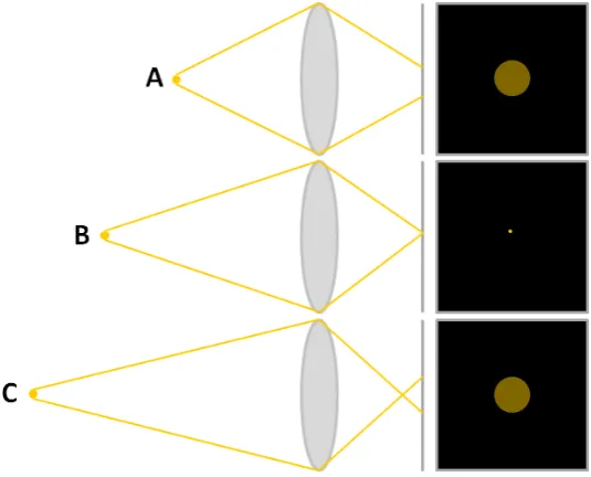
it is considered to be out of focus, or defocused. In optics, focus is defined as the point at which light rays originating from a point on an object converge. Thus, if an image point is in-focus, light from the point will be well converged on the image plane, whereas light from defocused image points will not. This is illustrated in Figure 2.1, where the object point that is perfectly in focus is known as the point of critical focus (B).
Figure 2.1: Light rays from a focused point in a given scene (B) converge on the image plane to form a point, whereas light rays from defocused points (A and C) do not converge and thus form a spot on the image plane.
2.2.2 Thin Lens Law
Modelling a camera as an image plane and a thin convex lens with a focal lengthf, the relationship between a focused point in a scene and the position of its focused point on the image plane can be derived by using the optical geometry shown in Figure 2.2. Two pairs triangles are identified as shown in Figure 2.3.
Using the law of similar triangles gives the following equations
I O =
v
u , (2.1)
and
I O =
v−f
f , (2.2)
Figure 2.2: Lens system showing central, parallel and focal rays from focused object point and corresponding image, wheref is the focal length,I is the the image size,
O is the object size, u the distance from the lens to the object and v the distance from the lens to the image.
(a) (b)
Figure 2.3: Two similar triangles within the lens system shown in Figure 2.2.
are the distances from the lens to the object and image, respectively. Substituting Equation 2.1 in Equation 2.2 gives
u v =
f
v−f . (2.3)
thus giving the well known thin lens formula for a focused point: 1
f =
1
u +
1
v . (2.4)
2.2.3 Circle of Confusion
the image plane, but instead upon an optical spot. This spot is known by a variety of names including ‘circle of indistinctness’, ‘blur circle’, ‘blur spot’ and ‘circle of confusion’. For the purposes of this thesis it will be referred to as the the circle of confusion (CoC). The relationship between the diameter of the CoC and the depth is shown by [Pentland, 1987]. Rearranging the thin lens law (i.e., Equation 2.4) in terms ofu gives
u= vf
v−f . (2.5)
For a particular lens system, the focal length f is constant. Assuming that the distance between the lens and the image plane is fixed atv=v0, and the distance at which a point will be in perfect focus is atu=u0, gives
u0=
f v0
v0−f
. (2.6)
Figure 2.4 illustrates the case when the distance of the object from the lens, u, is greater than the critical point of focus,uo with a lens of radiusr. This gives a CoC
with radiusσ.
Figure 2.4: Lens system with fixed values v0, u0 and f, when the distance of the object from the lens,u, is greater than the critical point of focus,u0. This gives the resultant circle of confusion of radiusσ.
Using the law of similar triangles, it can be shown that
r v =
σ v0−v
. (2.7)
u= f rv0
rv0−f r+f σ
. (2.8)
It can equally be shown that for objects closer to the lens than the critical focus point
u= f rv0
rv0−f r−f σ
, (2.9)
which gives the general equation
u= f rv0
rv0−f r±f σ =
(
+ if u > u0
− if u < u0
, (2.10)
or
u= f v0
v0−f ±σFN
= (
+ if u > u0
− if u < u0
, (2.11)
where FN is the f-number of the lens. This shows depth to be an indicator for
defocus. Lai [Lai et al., 1992] rewrites the equation to more clearly show the rela-tionship. Assuming that for a given lens systemf,v0 andFN are all constant, then
Equation 2.11 can be written as:
u= P
Q±σ . (2.12)
whereP =f v0/FN,Q= (v0−f)/FN, and P and Q are constant for a given camera
system. When a point is in perfect focus at the critical focus point, the amount of defocus, σ, will be zero (u0 = P/Q). The formula shows that the CoC gradually increases as the object point moves either deeper (i.e., further away) or shallower (i.e., nearer) to the lens than the critical focus pointu0.
2.2.4 Depth of Field
scene. Figure 2.5 shows an example whereby an identical scene is captured twice by a camera. The DoF of image (b) is lower than that of (a), and thus the background and parts of the object further from the lens appear blurred.
(a) (b)
Figure 2.5: Images of an identical scene captured using lens systems with a different DoF: (a) with an aperture off /32 and (b) with a relatively large aperture of f /5.
It can be seen from Equation 2.11 that a number of variables can be altered to produce an image with a low DoF, i.e. a larger CoC for a given distance from the critical focus point. Photographers will usually either use a larger aperture or lens with a longer focal length in order to achieve the effect. Figure 2.6 (a) and (b) respectively show the effect of using a large and a small aperture. It can be seen that a smaller aperture results in smaller CoCs, and thus a greater DoF, and vice versa.
2.2.5 Low Depth of Field Photography
Figure 2.6: The effect of aperture size on depth of field. Lens system (A) shows the effect of a larger aperture on CoC size (and thus DoF) whilst (B) shows that of a smaller aperture.
2.3
Image Segmentation
In computer vision, image segmentation is the process of dividing a digital image into multiple parts or segments. This is typically to simplify or change the appear-ance of the image to allow meaningful data to be more more easily extracted or analysed. Pixels are grouped into non-overlapping segments which share a similar characteristic or property, such as colour, intensity or texture. The union of these segments forms the entire image, and no two adjacent segments will have the same property. Segmentation is more formally defined in [Pal and Pal, 1993].
For a segmentation method where F is the set of all pixels and P( ) is a characteristic value assigned to a group of similar connected pixels if they fulfil a logical criteria (known as the uniformity predicate), then segmentation is the partitioning of the setF into a set of connected subsets or regions (S1, S2, S3, ..., Sn)
such that
n
[
i=1
Si =F withSi∩Sj =∅, i6=j . (2.13)
The uniformity predicate P(Si) = true for all regions Si, and when Si is
adjacent toSj then P(Si ∪Sj) = false. This remains true for all types of images,
(a) (b)
Figure 2.7: Use of low DoF: (a) in film production, and (b) in portrait photography.
2.4
Object Segmentation
Object segmentation is a specific case of image segmentation whereby the aim is to divide the image into two different areas, the object of interest (OoI) and the background. This is known as a binary segmentation. Some algorithms also generate a third ambiguous region along object boundaries. Object segmentation can be more problematic than image segmentation as a given object may have different properties such as colour or texture across its surface. It my also contain multiple internal contours (e.g., edges within an object) making object segmentation via edge detection a difficult task.
Segmentations can be divided into three different categories: those that are performed entirely by the user (i.e., manual segmentations); those that deal with a specific type of image or object, thus reducing the unknowns and allowing for au-tonomous segmentation methods (i.e., unsupervised segmentations); and those that use human input to guide or refine a segmentation (i.e., supervised segmentations) and thus can function with a wider or general range of objects and scenes.
2.4.1 Manual Segmentation
2.4.2 Unsupervised Segmentation
Creating a general unsupervised segmentation method is notoriously difficult due to the sheer range and variation in image characteristics and is considered to be an unsolved problem. Autonomous segmentation methods therefore require some form of a priori knowledge about the image. This could be information about the background, or the object to be segmented, or even more general image properties. For example, the method this thesis presents in Chapter 4 uses the fact that input images will have a low DoF, and that the OoI will be in clear focus, in order to perform autonomous segmentations.
By limiting the potential variations from image to image, unsupervised seg-mentations can form part of larger autonomous systems. For example, one well documented application is in automated-picking robots.
2.4.3 Supervised Segmentation
Supervised segmentations combine the most efficient parts of manual and automatic segmentations. A HVS can identify very quickly which parts of an image are of interest and this additional information allows a segmentation algorithm to function quickly and accurately. The user input in supervised methods is generally given in one of the following three ways:
1. Specification of an initial boundary, or parts of a boundary. This initial con-tour then evolves to the desired object boundary and is used in segmentation methods based on the active contours algorithm [Kass et al., 1988].
2. Denotation of a small set or sets of pixels that belong to the object or segment of interest, this is sometimes known as a ‘seed’. In some methods the user will also specify a set of pixels that belong to the background of the image. Well known techniques such as GraphCuts [Boykov and Jolly, 2001] and seeded region growing methods often use this kind of user input.
3. Specification of points along an OoI’s boundary. These points are connected to form a contour which then ‘snaps’ to the desired object’s boundary. This form of input is used in methods such as intelligent scissors [Mortensen and Barrett, 1995].
given enough time, a user can repeatedly refine the segmentation until a ‘perfect’ result is obtained.
2.5
Segmentation Methods
Image segmentation is a popular and well researched field, and thousands of segmen-tation methods have been presented in literature [McGuiness and O’Conor, 2010]. Aside from being categorised on levels of user input, methods can be further subdi-vided into two areas: edge based and region based methods.
Edge detection is an entire field of image processing in itself, but can form the basis of segmentation techniques. Edge-based segmentation methods generally use some form of edge operator or filter followed by a thresholding to obtain the contours in an image. Enclosed regions are considered to be separate segments as they lack continuity with adjacent regions and can be identified by simple ‘fill’ operations. Broken contour lines, for example caused by blurring, will result in failed segmentations and thus such methods tend to involve some form of line-linking operation.
For the task of binary object segmentation, region based techniques are more applicable. This is because edge detection methods cannot produce binary segmen-tations of objects with multiple internal contours. This section discusses some of the broad concepts that are the basis for many segmentation methods.
2.5.1 Thresholding
Thresholding is one of the simplest methods for image segmentation. In its most basic form it assigns all pixels with intensity values (F) above a certain level as object and those below this threshold,α, as background, i.e.,
ifF(x, y)≥α F(x, y) = 1 (object)
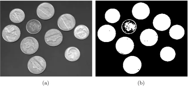
else F(x, y) = 0 (background) . (2.14) The threshold can be given manually or calculated automatically. For example Otsu’s method [Otsu, 1979] automatically generates a threshold for a binary seg-mentation by minimising the intra-class variance, as shown in Figure 2.8.
(a) (b)
Figure 2.8: Segmentation of an initial image (a) using a threshold automatically generated via Otsu’s Method to produce a binary segmentation (b).
subimages. These are considered separately and optimal thresholds for each subim-age are found. These calculated thresholds are used to interpolate the threshold for each individual image pixel. More current approaches use a less computationally in-tensive local thresholding approach, where the threshold for a pixel is determined by the values of pixels in its neighbourhood. For a example, a simple local thresholding could use the mean of neighbouring pixels to calculate a threshold:
ifF(i, j)≥M−C F(i, j) = 1 (object)
else F(i, j) = 0 (background) . (2.15) whereC is a constant andM is the mean of pixels belonging to the neighbourhood of size (2N+ 1)×(2N+ 1) given by
M = 1 (2N + 1)2
i+N
X
x=i−N j+N
X
y=j−N
F(x, y). (2.16)
The size of the neighbourhood used greatly impacts on the performance of the segmentation method.
2.5.2 Histograms
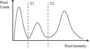
Grey level histograms can also be used to determine thresholds for binary segmen-tations. Once peaks in a histogram have been identified, a threshold can be set at the minima between them, as shown in Figure 2.9.
Figure 2.9: Histogram of the intensity/grey level in a image. The selected threshold, T1, corresponds to the minimum between the two peaks.
histogram is computed from all image pixels, and peaks and troughs are identified to group similar pixels, for example as shown in Figure 2.10. Such a method can easily be extended to grouping pixels with similar colours rather than grey levels.
Figure 2.10: Histogram of the intensity level in a image with three groupings of pixels. Threshold levels correspond to the minima between peaks.
Compared to some other segmentation techniques, a histogram is computa-tionally very efficient, requiring only a single pass of the image. If the groupings of pixels are not very distinctive then difficulties can arise in selecting appropriate thresholds. More complex methods use further histograms to recursively break down clusters of similar pixels into smaller groupings. Whilst effective at grouping similar colour pixels, a binary object segmentation via histogram may not be possible if an object is not of a uniform colour.
2.5.3 Clustering
[image:34.595.228.414.340.441.2]be picked randomly or seeded. The algorithm then follows the following iterative process:
1. Each pixel is assigned to a cluster which minimises the distance between the cluster centre and the pixel.
2. Cluster centres are re-calculated by averaging all the pixels within the cluster. These two steps are repeated until there are no further changes in the mem-bership of the clusters. The distance is commonly defined as either the square or absolute difference between a pixel and the cluster centre, and can be based on colour, intensity, texture, or a weighted combination of these factors. Figure 2.11 shows an image segmented using a K-means algorithm withK= 16.
(a) (b)
Figure 2.11: Colour segmentation of an image (a) using a K-means algorithm with 16 clusters to produce a colour segmentation (b).
2.5.4 Region Growing
Region growing algorithms often make use of user defined seeds [Adams and Bischof, 1994]. In its simplest form, a seed is placed in each object or region to be segmented. From these starting points, regions are grown iteratively from all unallocated neigh-bouring pixels. The intensity or hue of the neighneigh-bouring pixel that is most similar to the mean of the region being grown is allocated to that region. This is repeated until all pixels are allocated to a region.
Adjacent regions can be merged under some criteria, for example sharpness of region boundaries. A harsh criterion can create a fragmented segmentation whereas a lenient one could overlook blurred boundaries and oversimplify the segmentation.
2.5.5 Split and Merge Algorithms
Region merging methods address the problem of image segmentation from the bot-tom up. Every pixel is considered to be a seed. If two neighbouring pixels are the same, or similar enough according to some criterion, then they are merged into a single region. Likewise, if properties of two adjacent regions are similar enough to each other, they will be merged. This process continues until no further merging is possible. These kinds of algorithms are computationally very intense. Split and merge algorithms, proposed by Horowitz [Horowtiz and Pavlidis, 1974], are much more efficient and start from the top downwards.
A quadtree structure is generally used for the splitting process. The entire image is considered to be a single region. If this region is uniform (or if all pixels within the region have sufficient similarity) then the region is left as it is. If the pixels in the region are non-homogeneous (or outside of some range or threshold of conformity) it is then subdivided into four quadrants, i.e., the child regions. The process is then repeated for each of these child regions, i.e., the conformity of the pixels is checked which determines whether the region will be split again. These subdivisions are continued until no further splits occur or the resolution of the quadtree is reached. The merging algorithm can then proceed, merging regions from the bottom up. Starting with these small regions rather than single pixels means that split-merge methods are significantly more efficient than pure merge algorithms.
2.5.6 Watershed Transformation
In practice watershed transform tends to be performed on the morphological gradient of the image, not the greyscale image. This generates watershed lines along the points of intensity discontinuity, most likely edges, meaning the regions or basins will correspond to objects, or object regions within an image.
2.5.7 Active Contours
The general principle behind an active contours algorithm is that an initial curve or snake evolves to try and minimise an energy function, drawing it towards an object boundary [Kass et al., 1988]. Representing the snake parametrically by v(s) = (x(s), y(s)), the energy function can be written as
Esnake∗ = Z 1
0
Esnake(v(s))ds
= Z 1
0
[Einternal(v(s)) +Eimage(v(s)) +Econstraints(v(s))] ds(2.17)
where Einternal is the internal energy of the curve due to bending, Eimage is the
force pulling the contour towards salient image features andEconstraintsare external
constraints imposed upon the curve by the user.
Active contours models can either be parametric snakes or geometric snakes. Parametric snakes are represented by splines and the contour evolution is only per-formed on specific points along the contour. They have the disadvantage of not being able to split the contour to detect multiple objects without manual interven-tion and, unless the initial curve is close to the object boundary, can converge on non-object points [Hou and Han, 2005].
Figure 2.12: Level set method: (bottom row) the evolving level set function of a 3D dark grey object and a 2D light grey image plane; (top row) the corresponding contour curves of the object regions on a 2D image plane are the zero-level set values of the evolving object surface.
by a gradient and is very robust to noise.
One of the main criticisms of active contour algorithms is that they are computationally intensive, especially when dealing with large images. This is par-ticularly true of level set methods. A number of implementations can be used to increase speed. The sparse field method [Whitaker, 1998] is a narrow band level-set implementation which substantially reduces the number of computations required per iteration by only performing calculations near the zero level set. Other criti-cisms of active contours are that methods tend to be very dependent on having a good initial contour, which is why they are commonly defined by the user. In some implementations there are also risks of the evolving boundary becoming stuck in local minima.
2.5.8 Graph Partitioning Methods
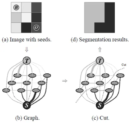
A min-cut algorithm (aiming to minimise the cost of links cut) categorises pixels as either object or background, thus segmenting the image. This process is illustrated in Figure 2.13.
Figure 2.13: Example of a simple segmentation of a 3x3 image where T is the background terminal and S the object terminal. ‘B’ and ‘O’ denote background and object seeds, respectively. Figure is adapted from [Boykov and Jolly, 2001].
2.5.9 Conclusion
Chapter 3
Focus Assessment
3.1
Introduction
Research into the focus of an image is not an uncommon theme. This can vary from assessing the focus of an entire image to identifying regions of different focus within a given image. However, the objective is the same, namely to determine whether the image, or parts of the image, have undergone some kind of blurring operation as a result of being outside of the DoF, as discussed in Chapter 2. Assessments of whole images can be used to determine whether images of a given scene are focused more or less than each other, for example when the distance of the image plane from the lens is changed. Focus assessment of the regions within an image can be used to obtain further information about a scene, e.g., to identify objects, or estimate the depth of regions within a calibrated image. The most common way of determining a focus value of a pixel is by determining how much it contrasts with its neighbouring pixels, i.e., how blurred the section of the image is.
produced.
Other applications include image fusion [Huang and Jing, 2007], where focus assessments are used to merge two images that focus on different parts of a scene in order to create one fully focused composite image. This can also be applied in microscopy so that structures at different levels are in focus in the composite image. Defocus can also be used to estimate the depth of pixels in an image [Pentland, 1987] which in turn can be used to perform 3D reconstruction of surfaces [Nayar and Nakagawa, 1994].
The premise behind the object segmentation method presented in this thesis is that by limiting the type of image to be processed to those with a low DoF, an autonomous method can be created. Assuming that an image generated from a camera system has focused on the OoI within a given scene, the background pixels of the image will be less sharp when compared to object pixels. A focus assessment allows the different regions, e.g., background and object, to be differentiated by some segmentation method. This chapter is primarily concerned with the selection of a suitable assessment to create a focus map, and is organised as follows: Section 3.2 briefly describes the most common way of modelling defocus. Section 3.3 provides an overview of the seminal focus assessment methods, dividing them into three different categories; statistical, derivative, and wavelet based methods. Example focus maps are shown for a number of different assessments. Section 3.4 evaluates the suitability of a range of different focus assessment methods for the problem of object segmentation from low DoF images. Section 3.5 considers the effects of image resolution on the performance of the focus assessment methods. Finally, Section 3.6 proposes a multiscale variation of a wavelet based focus assessment. Some focus maps generated using this method are shown in Section 3.7. In Section 3.8, the chapter is concluded.
3.2
Modelling Defocus
The point spread function (PSF) describes how an imaging system will respond to an object point, i.e., the blurring operation an object point undergoes when an image is formed. The relationship between the actual or original scene f(x, y) and the corresponding captured imageg(x, y) can be described by the following convolution [Jain, 1998]:
whereh(x, y) is the PSF of blurring and has the characteristics of a low-pass filter. Autofocusing algorithms seek to minimise blur such thatg(x, y) ≈f(x, y). As the blurring caused by defocus is modelled as a low-pass filter, most focus assessments measure high-frequency components in an image, to detect areas less affected by blurring.
3.3
Focus Assessment Methods
The basic premise behind most focus assessment methods is that focused images will contain more information, or detail, than defocused or blurred images. Detecting the presence of this detail, shown as high frequency components, is key to assessing an image’s level of focus. As such, it is common for methods to rely on edge information, where the contrast between neighbouring pixels will be greatest. As focused images will have sharp edges, they will contain more high frequency content than their equivalent in a defocused image.
This premise leads to a number of issues. If the focus differential between the background and foreground is small, then some background contours may have higher frequency components than internal parts of the focused OoI. This is partic-ularly true of objects which are mostly homogeneous, or have weak textures. This is because despite being within the DoF, if there is no contrast between adjacent pixels (for example in a mono-colour plastic object where the illumination is equal on all parts) then the object will behave the same as a defocused region, having no high frequency components. Only the region boundaries can be differentiated.
Other potential problems in assessing the focus of an image include artefacts such as light glare or flash reflections. These can potentially create artificial high frequency components in the otherwise less sharp background.
The size or resolution of an image will also have an effect on focus assessment. Whilst in images of a small size (which is defined in this thesis as having height and width in the order of hundreds, not thousands of pixels), or low resolution, edges are likely to be the most prominent and useful factor in determining focus. For larger scales or higher resolution images, the internal contours and texture have significant effect.
3.3.1 Statisical Methods
Statistical methods are generally applied to automatic focusing problems. They work on the basis that focused images will have more information than defocused images. Rather than assessing focus on pixel level, they assess the whole image. Thus they are useful in determining the comparative focus between images of the same scene, hence their use in autofocusing algorithms. They tend to be more robust to image noise than other types of focus assessment methods.
Variance
The variance algorithm [Groenand et al., 1985; Yeo et al., 1993], sums the square in the difference in pixel intensitiesi(x, y) from the mean intensity. The focus value is
Fvariance=
1 H.W X Height X W idth
(i(x, y)−µ)2 , (3.2) whereHis the image height,W is the image width andµis the mean pixel intensity. Squaring the difference amplifies larger difference in pixel intensities from the mean.
Normalised Variance
The normalised variance algorithm [Groenand et al., 1985; Yeo et al., 1993] factors the mean intensity into the final focus value. This allows the focus of images of dif-ferent scenes to be compared as changes in average image intensity are compensated for. The focus value is
Fvariance=
1 H.W.µ X Height X W idth
(i(x, y)−µ)2 , (3.3) whereHis the image height,W is the image width andµis the mean pixel intensity. As with the variance method, squaring the difference amplifies larger difference in pixel intensities from the mean.
(a) (b)
Figure 3.1: Low DoF image taken from video footage (a), and the same image having undergone a blurring operation (b). The focus values calculated using the normalised variance for the images are 0.0657 and 0.0594, respectively.
Range Algorithm
Other statistical algorithms make use of histograms, h(i), to analyse the distribu-tions of intensities within an image. The range algorithm [Firestone et al., 1991] computes the difference between the highest and lowest intensity levels, i.e., the focus value is
Frange =maxi(h(i)>0)−mini(h(i)>0) . (3.4)
The premise being that blurring will attenuate any extreme values in pixel intensity.
Entropy
The entropy algorithm [Firestone et al., 1991], as with all the statistical methods, assumes that images that are in focus contain more information than those that are not. Utilising a histogram the focus value is
Fentropy =−
X
intensities
pi.log2(pi) , (3.5)
wherepi =h(i)/(height×width) is the probability that a pixel has an intensity of
i, and height and widthare the dimensions of the image. 3.3.2 Derivative Methods
from of convolution mask to apply a high pass filter and obtain a map of the deriva-tives, giving an indication of the focused areas in the image.
The derivative methods in this section sum the results of the convolution to obtain a focus value for the image. In order to produce a pixel based focus assessment of the image, the summing is not performed and instead the results of the convolution are used as a focus intensity map. This makes such methods more suitable as an initial stage in a segmentation method than the statistical methods in Section 3.3.1.
Tenengrad
The Tenengrad focus operator [Tenenbaum, 1970] applies vertical and horizontal Sobel operators to the image. In order to compute the focus value of a pixel, the square of the results of the convolution are summed within an (2N + 1)×(2N+ 1) window centred around the pixel to be assessed, i.e.,
FT enengrad(i, j) = i+N
X
x=i−N j+N
X
y=j−N
Sx(x, y)2+Sy(x, y)2, (3.6)
where Sx(x, y) and Sy(x, y) are the results of the convolution of the image with
the horizontal and vertical Sobel operators, respectively (i.e., along the x and y
directions, respectively).
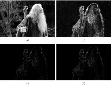
Figure 3.2 shows an example of the Tenengrad method being applied to a DoF image of a wizard against a forest background. The corresponding focus intensity map generated is shown in Figure 3.2(b).
(a) (b)
Modified Laplacian
Designed to cope with weakly textured images, the modified Laplacian (ML) oper-ator [Nayar and Nakagawa, 1994] sums the absolute values of the convolution of the image with the Laplacian operators, giving the focus value
FM L(i, j) =|Lx(x, y)|+|Ly(x, y)|, (3.7)
where Lx(x, y) and Ly(x, y) are the results of the convolution of the image with
the horizontal and vertical Laplacian operators (Lapx and Lapy), respectively (i.e.,
along thex and y directions, respectively), with
Lapx=
h
1 −2 1 i
, Lapy =
1
−2 1
.
The Laplacian methods were developed to measure focus at each image point in order to estimate depth as part of a shape from focus system. Figure 3.3 shows the ML method being applied to the image of the wizard.
(a) (b)
Figure 3.3: Low DoF image taken from video footage (a), and the corresponding focus intensity map generated using the ML method (b). The image has had its intensity enhanced by a factor of 3 for clarity.
Sum Modified Laplacian
The sum modified Laplacian (SML) method sums the results of the ML method within a local window to obtain the focus value
FSM L(i, j) = i+N
X
x=i−N j+N
X
y=j−N
whereFM L(x, y) is the convolution of the image with the modified Laplacian
oper-ator.
(a) (b)
Figure 3.4: Low DoF image taken from video footage (a), and the corresponding focus intensity map generated using the SML method (b). The image has had its intensity enhanced by a factor of 3 for clarity.
Energy Laplace
The Energy Laplace method [Subbarao et al., 1993] is another kernel based focus assessment. It was proposed as a recommended measure for camera autofocusing systems. It uses the operator
L=
−1 −4 −1
−4 20 −4
−1 −4 −1
to give the focus value
FEL(i, j) = i+N
X
x=i−N j+N
X
y=j−N
C(x, y)2, (3.9)
(a) (b)
Figure 3.5: Low DoF image taken from video footage (a), and the corresponding focus intensity map generated using the Energy Laplace method (b). The image has had its intensity enhanced by a factor of 3 for clarity.
Daugman
Originally applied in the the field of iris recognition to select optimal images, Daug-man’s method [Daugman, 2004] uses the following 8×8 focus assessment kernel:
D=
−1 −1 −1 −1 −1 −1 −1 −1
−1 −1 −1 −1 −1 −1 −1 −1
−1 −1 3 3 3 3 −1 −1
−1 −1 3 3 3 3 −1 −1
−1 −1 3 3 3 3 −1 −1
−1 −1 3 3 3 3 −1 −1
−1 −1 −1 −1 −1 −1 −1 −1
−1 −1 −1 −1 −1 −1 −1 −1 .
Its convolution with the image gives the focus value
FDaugman(i, j) =C(x, y), (3.10)
(a) (b)
Figure 3.6: Low DoF image taken from video footage (a), and the corresponding focus intensity map generated using Daugman method (b). The image has had its intensity enhanced by a factor of 3 for clarity.
Wei
Wei presents an improved focus assessment [Wei et al., 2006] over Daugman’s method, using a smaller 5×5 kernel to improve computational efficiency, i.e.,
W =
−1 −1 −1 −1 −1
−1 2 2 2 −1
−1 2 0 2 −1
−1 2 2 2 −1
−1 −1 −1 −1 −1
.
Its convolution with the image gives the focus value
FW ei(i, j) =C(x, y), (3.11)
(a) (b)
Figure 3.7: Low DoF image taken from video footage (a), and the corresponding focus intensity map generated using Wei’s focus assessment kernel (b). The image has had its intensity enhanced by a factor of 3 for clarity.
Kang
Kang’s focus assessment kernel [Kang and Park, 2005; Kang, 2006] is another 5×5 operator, i.e., K =
−1 −1 −1 −1 −1
−1 −1 4 −1 −1
−1 4 4 4 −1
−1 −1 4 −1 −1
−1 −1 −1 −1 −1 .
It is again proposed for use within the field of iris recognition. Its convolution with the image gives the focus value
FKang(i, j) =C(x, y), (3.12)
where C(x, y) is the convolution of the image with operator K. Figure 3.8 shows the result of Kang’s kernel being applied to a low DoF image.
3.3.3 Wavelet Methods
A series of focus measures utilising wavelets is proposed in [Yang and Nelson, 2003a,b]. The focus value is used as a cue for the segmentation of low DoF mi-croscopic images via a graph partitioning method. The Daubechies 6 wavelet filter is used to divide the image into four subband imagesWLL,WHL,WLH and WHH,
(a) (b)
Figure 3.8: Low DoF image taken from video footage (a), and the corresponding focus intensity map generated using Kang’s focus assessment kernel (b). The image has had its intensity enhanced by a factor of 3 for clarity.
highpass filtering followed by lowpass filtering. The focus measures are as follows:
Wavelet 1
Fwavelet1=|WHL(x, y)|+|WLH(x, y)|+|WHH(x, y)| (3.13) Wavelet 2
Fwavelet2 = (|WHL(x, y)| −µHL)2+ (|WLH(x, y)| −µLH)2+ (|WHH(x, y)| −µHH)2
(3.14) whereµis the mean of a subband image computed using absolute values.
Wavelet 3
Fwavelet3 = (WHL(x, y)−µ¯HL)2+(WLH(x, y)−µ¯LH)2+(WHH(x, y)−µ¯HH)2 (3.15)
where ¯µis the mean of a subband image computed without using absolute values. Figure 3.9 shows the three methods being applied to a low DoF image of a wizard against a wooded background.
3.4
Evaluation of Focus Measures
(a) (b)
[image:52.595.124.518.108.406.2](c) (d)
Figure 3.9: Low DoF image taken from video footage (a), and the corresponding focus intensity map generated by the wavelet 1 method (b), the wavelet 2 method (c) and the wavelet 3 method (d). The images have been contrast-enhanced by a factor of 3 for clarity.
resolution (HR) test images as shown in Figure 3.10 and eight lower resolution (LR) test images as shown in Figure 3.11 with clear focus differentials between the background and in-focus objects (i.e., the OoIs) are manually segmented to obtain their ground truth. The number of pixels along each of the dimensions of a HR image and a LR image is of the order of thousands and hundreds, respectively.
The focus assessment methods are applied to the images, and the properties of the resulting range of focus values for the object and background regions recorded. The following two criteria are used to determine the best measure:
¯
Fbackground F¯object (3.16)
σbackground σimage (3.17)
where ¯Fbackgroundand ¯Fobjectare respectively the mean focus value of the background
devi-Figure 3.10: High resolution test images with focus differentials between OoI and background.
Figure 3.11: Low resolution images with focus differentials between OoI and back-ground.
ation of the background and image focus values. The value of ¯Fbackground should
be low compared to ¯Fobject, thus the higher the ratio ¯Fobject/F¯background the better
the measure. σbackground should be as small as possible when compared to σimage,
as the background should be relatively homogeneous. The lower σbackground is, the
[image:53.595.122.516.361.575.2]to focus values of anomalous background pixels. The focus measures are ranked against each other for both criteria and given a score (the sum of the ranking for the two criteria) for each of the test images, i.e.,
Score=RankingF¯object/F¯bkgnd+Rankingσbkgnd/σimage (3.18)
where a subscript denotes the criterion used for the ranking. The average score for each focus measure is obtained allowing the overall ranks to be calculated. This is performed separately for the HR and LR images, as summarised in Table 3.1.
Method ScoreHR RankHR ScoreLR RankLR
Daugman 7.500 4 19.625 10
Energy Laplace 6.500 3 3.000 1
Kang 13.375 7 15.000 8
ML 17.125 9 11.875 6
SML 16.375 8 12.375 7
Tenengrad 2.125 1 7.500 4
Wavelet 1 19.875 10 11.750 5
Wavelet 2 6.125 2 6.875 3
Wavelet 3 9.875 5 4.625 2
Wei 11.125 6 17.375 9
Table 3.1: Evaluation of focus assessment methods, where the subscripts denote the types of images processed.
Table 3.1 shows that the focus assessment method which gives the most suitable focus measure for the HR images is the Tenengrad method, followed by the wavelet 2 method and the Energy Laplace method. For the LR images the highest ranked focus assessment method is the Energy Laplace, followed by Wavelet 3 and Wavelet 2. Thus, there is no focus assessment method that is best for both sets of images.
as well as weaker values for the areas within an object boundary, i.e., object edges are amplified while most other areas are attenuated. This makes the segmentation of the OoI a more challenging prospect.
The Wavelet 3 method is ranked highly in the focus assessments for the LR images and the nature of the wavelet transform means that the method can be adapted for HR images. We therefore propose in Section 3.6 a focus assessment based on the Wavelet 3 method that provides a measure suitable for use with active contours on any image resolution.
3.5
Focus Assessment and Image Resolution
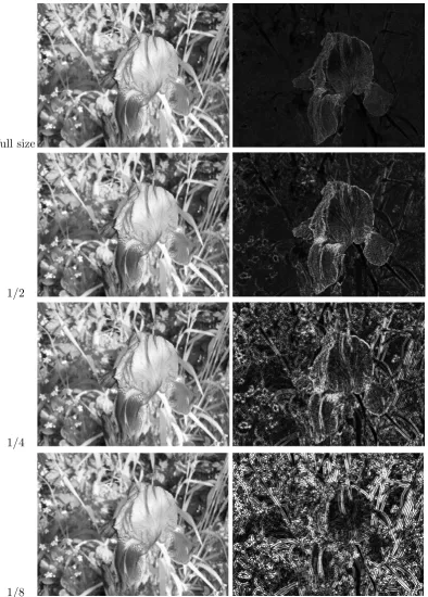
It is important to note the effect that image resolution, or image size, has on focus assessments. In Chapter 2, DoF is defined as the region for which the diameter of the CoC is less than the resolution of the display medium - in this case the resolution of the image. By reducing the resolution of the image, the diameter of the CoC becomes smaller when compared to pixel size. This means that lower resolution images are likely to return higher values when their focus is assessed.
full size
1/2
1/4
[image:56.595.127.522.106.657.2]1/8
level of decomposition can be chosen that suits the image to be segmented.
(a) (b)
Figure 3.13: The effect of a reduction in image resolution on background contours.
3.6
Proposed Focus Assessment Method
A wavelet based focus measure which reflects the strength of the high frequency details is proposed in [Yang and Nelson, 2003a]. The method considers the first level of wavelet decomposition only and is given by (3.15). To extend the method for use with images of any resolution, (3.15) is modified to
F(x, y) =|DH(x, y)−µDH|+|DV(x, y)−µDV|+|DD(x, y)−µDD|, (3.19)
where DH, DV, and DD are the reconstructed detail coefficients (horizontal, vertical and diagonal) for the wavelet decomposition of the image at a levelN, andµDH,µDV
andµDD are the mean values of each reconstructed subband. The modulus is taken
as opposed to squaring the value as in Equation 3.15 to avoid object boundaries from becoming too dominant in the focus map.
For very high resolution images, taking the detail coefficients from further levels of decomposition aids in segmentation. This is because texture changes and contours of focused OoIs in high resolutions will transition over a number of pixels. Pixels will therefore contrast significantly less with their neighbours than if the image scale were smaller, leading to smaller values being returned in the focus assessment. By taking the detail coefficients from a lower level where this is the case, the performance of segmentation algorithms can be improved as it will be significantly easier to differentiate the object from the background.
intrinsically linked. The segmentation method was therefore developed simultane-ously with the focus assessment method. This allowed the methods to be somewhat tailored to each other. An initial version of the object segmentation method pre-sented in Chapter 4 based on the active contours algorithm was utilised to help determine the appropriate level of wavelet decomposition.
The focus assessment using (3.19) is first performed at level 1, i.e, N = 1. If the standard deviation (Std) of the image’s focus values is below a thresholdT, i.e., there is no significant difference between the background and object pixels, the process is then repeated atN = 2. If the Std is also belowT at this level, the detail coefficients will be taken from the level 3 wavelet decomposition. This is unlikely to occur in images that are not of high resolution. If the standard deviation of the focus map is still beneath the threshold it is assumed that the OoI is either weakly textured or has a very small area and the values at N = 3 are used. Table 3.2 shows data used to determine the optimum value for the threshold, i.e.,T = 0.0105. Comparing the Std of focus values with the percentage of correctly segmented pixels (found using manually generated ground truths) using the active contours algorithm enables the threshold to be chosen experimentally.
Image Level Image Std Correctly Segmented
Flower 1 0.0069 35.7
2 0.0119 98.7
3 0.0165 97.3
4 0.0249 91.9
Soft Toy 1 0.0074 95.5
2 0.013 98.9
3 0.0138 98.8
4 0.0142 97.2
Watch 1 0.0047 34.6
2 0.0100 91.2
3 0.0150 99.3
4 0.0209 97.4
Plant 1 0.0057 28.1
2 0.0085 36.1
3 0.0105 98.9
4 0.0173 98.1