Munich Personal RePEc Archive
Spatial panel data models with structural
change
Li, Kunpeng
Capital University of Economics and Business
21 March 2018
Online at
https://mpra.ub.uni-muenchen.de/85388/
Spatial panel data models with structural changes
∗Kunpeng Li
International School of Economics and Management Capital University of Economics and Business
March 22, 2018
Abstract
Spatial panel data models are widely used in empirical studies. The existing theories of spatial models so far have largely confine the analysis under the assump-tion of parameters stabilities. This is unduely restrictive, since a large number of studies have well documented the presence of structural changes in the relationship of economic variables. This paper proposes and studies spatial panel data models with structural change. We consider using the quasi maximum likelihood method to estimate the model. Static and dynamic models are both considered. Large-T and fixed-T setups are both considered. We provide a relatively complete asymptotic theory for the maximum likelihood estimators, including consistency, convergence rates and limiting distributions of the regression coefficients, the timing of structural change and variance of errors. We study the hypothesis testing for the presence of structural change. The three super-type statistics are proposed. The Monte Carlo simulation results are consistent with our theoretical results and show that the max-imum likelihood estimators have good finite sample performance.
Key Words: Spatial panel data models, structural changes, hypothesis testing, asymptotic theory.
JEL:C31; C33.
∗This paper was presented at Advanced Econometric Forum of Wuhan University, March 19, 2018. I
1
Introduction
Since the seminal works of Cliff and Ord (1973) and Ord (1975), spatial econometric models have received much attention in the economic literature. A typical spatial au-toregressive model specifies that one’s outcome is directly affected by the outcomes of its spatial peers with some prespecified weights. With this particular specification, one has the chance to study the spatial interactions among a number of spatial units.
Spatial econometric models have been widely used in empirical studies. In microe-conomics, evoked by the influential work of Manski (1993), spatial models are one of primary tools to study the endogenous effects or peer effects, see e.g., Bramoullé, Djeb-bari and Fortin (2009), Calvó-Armengol, Patacchini and Zenou (2009), Lin (2010). In public economics, spatial models are widely used to study the competitions for tax and fiscal expenditure among local governments, see e.g., Lyytikäinen (2012), Chirinko and Wilson (2007), etc. In international economics, spatial models are popular in the studies of the spillover effects of foreign direct investment and the gravity model of trade, see e.g., Bode, Nunnenkamp and Waldkirch (2012). In urban economics, spatial models are used to study the diffusion process of housing prices, see Holly, Pesaran and Yamagata (2011). In finance, Kou, Peng and Zhong (2017) show that the traditional capital asset pricing model or the arbitrary pricing theory augmented with spatial interactions can improve the model fitting to the real data. Spatial econometrics models are also used to study some social issues. As one of motivating example in Anselin (1988), spatial term is introduced to capture the social patten among different districts arising from the sphere of criminals.
The literature has also witnesses rapid developments on the theory of spatial econo-metric models. Early development has been summarized by a number of books, includ-ing Anselin (1988) and Cressie (1993). Due to the presence of endogenous spatial term, the ordinary least squares (OLS) method cannot deliver a consistent estimation. Gen-eralized method of moments (GMM) and quasi maximum likelihood (ML) method are two popular estimation methods to address this issue. The GMM are studied by Kelijian and Prucha (1998, 1999, 2010), and Kapoor et al. (2007), among others. The ML method is investigated by Anselin (1988), Lee (2004), Yu et al. (2008) and Lee and Yu (2010), and so on.
sample with a small number of periods, it is still necessary to take into account struc-tural change as a conservative modeling step since one may be unlucky to have a sample at hand, which has experienced one or more typical structural change events, such as presidential adminstration switching, policy-regime shift, financial crisis, etc. It is well known that failure to account for the structural change, if it does exist, would cause inconsistent estimations and incorrect statistical inferences, resulting in misleading eco-nomic implications. Introduction of structural change in model is not just for correct statistical analysis concern. In some applications such as policy evaluations, specifying a structural change allows one to quantify the effect of policy intervention, which has its own independent interests.
This paper proposes and studies spatial panel data models in the presence of struc-tural change. We consider using the quasi ML method to estimate model. Our asymp-totic analysis first focuses on a static spatial panel model under large-Tsetup. The theory is next extended to a dynamic model, as well as to a model under fixed-Tsetup. We also consider the hypothesis testing issue on the presence of structural change. The supW, supLM, supLR statistics, which are based on the classical Wald, Lagrange Multipliers (LM) and Likelihood ratio (LR) tests, are proposed to perform this work. The asymptotic properties of these three statistics are investigated. To my best knowledge, this paper is the first to develop a relatively complete asymptotic theory on spatial panel data models with structural change.
A main difficulty of the current theoretical analysis is to establish the global proper-ties of the ML estimators. As far as I can see, one cannot directly apply the arguments well developed by the previous studies, such as Bai (1997), Bai and Perron (1998), Bai, Lumsdaine and Stock (1998), Qu and Perron (2007) and so forth, to the current model. The reasons are twofold. First, because of nonlinearity arising from the spatial lag term, we cannot concentrate out the regression coefficients from the objective function, which makes the arguments in Bai (1997) and Bai and Perron (1998) not suitable to our model. Second, the ML estimators would have biases due to the presence of incidental parame-ters. As a consequence, the ML estimators have two convergence rates, and which one is dominant depending on the values of N andT, where Nis the number of spatial units and T the number of periods. This feature makes the analysis of Bai, Lumsdaine and Stock (1998) much complicated since their analysis implicitly specifies the convergence rate. In addition, the particular identification issue in the spatial models requires some exclusive analysis to address it. In this paper, we develop a set of different and new arguments to establish the global properties, such as consistency and convergence rates. The proposed model is related with spatial econometrics and structural change mod-els, both of which have long histories and are very popular in empirical studies. As the mixture, we believe that the proposed model would inherit their popularity.
feature of this study is that the individual effects, which are the primary attractiveness of panel data models, are abstracted from the model. In addition, only supLR statistic is proposed in this study. In contrast, we propose three statistics. Among these three statis-tics, the supLM statistic is of more practical interests, since it only involves the estimator of the restricted model that is easier to compute. This can save much computation cost, especially when the sample size is large.
The rest of the paper is organized as follows. In Section 2, we propose a basic static model and write out the related likelihood function. The computation aspect of the model is also considered in this section. Section 3 lists the assumptions needed for the subsequent theoretical analysis. We also make a detailed discussion on the identification issue. Section 4 presents the asymptotic results. Section 5 makes an extension to the dynamic model. Section 6 gives the asymptotics under fixed-T setup. Section 7 con-sider the hypothesis testing for the presence of structural change. Section 8 runs Monte Carlo simulations to investigate the finite performance of the ML estimators. Section 9 concludes the paper.
2
Basic model and likelihood function
The model studied in this paper is a spatial autoregressive panel data model with a structural change, which is written as
Yt =α∗+ρ∗WNYt+̺∗WNYt✶(t≤[Tγ∗]) +Ztβ∗+Xtδ∗✶(t≤[Tγ∗]) +Vt, (2.1)
or equivalently
Yt =α∗+ (ρ∗+̺∗)WNYt+Ztβ∗+Xtδ∗+Vt, for t≤[Tγ∗],
Yt =α∗+ρ∗WNYt+Ztβ∗+Vt, for t> [Tγ∗],
whereYtis anN-dimensional vector of observations at timetfor the dependent variable. ρ∗WNYt and ̺∗WNYt✶(t ≤ [Tγ∗]) are two spatial terms. ✶(·) is an indicator function,
which is 1 if the expression in the brackets is true, and 0 otherwise. Zt andXtare N×p
andN×qobservable data matrices with p≥qat timetfor explanatory variables. Here the columns ofXtis a subset of those of Zt. The model is a pure change model if p=q;
and a partial change model if p > q. Our model specification implicitly assumes that
there is one break point and the structural change always appears in the spatial term. The model with multiple structural changes is also of theoretical interests and practical relevance. But such a topic is beyond the scope of this paper and is left as a future work. In addition, the model with the structural change only present in the coefficients ofXt is
simpler than model (2.1). The analysis of this simpler model can be easily obtained by slightly modifying the analysis of the current paper.
For notational simplicity, we introduce the following symbols:
Yt(γ) =Yt✶(t ≤[Tγ]), Yt(γ,γ∗) =Yt✶(t≤ [Tγ])−Yt✶(t≤[Tγ∗]),
Dt(ρ,̺,γ) = IN−ρWN−̺WN✶(t ≤[Tγ]), Dt∗ =Dt(ρ∗,̺∗,γ∗).
With these notations, the model now can be written as
D∗tYt =α∗+Ztβ∗+Xt(γ∗)δ∗+Vt.
Let θ = (ρ,̺,β′,δ′,γ,σ2)′. If V
t is normally and independently distributed with with
mean zero and varianceσ2IN, the gaussian log-likelihood function is
L(θ,α) =−1
2lnσ
2+ 1
NT
T
∑
t=1
ln
Dt(ρ,̺,γ)− 1
2NTσ2 T
∑
t=1
Xt(θ,α)′Xt(θ,α) (2.2)
where
Xt(θ,α) =Dt(ρ,̺,γ)Yt−α−Ztβ−Xt(γ)δ.
The first order condition forαgives
α(θ) = 1
T
T
∑
t=1
Dt(ρ,̺,γ)Yt− 1
T
T
∑
t=1
Ztβ−T1
T
∑
t=1
Xt(γ)δ.
Substituting the preceding formula into the likelihood function to concentrate outα, we have
Xt(θ) =]DtYt−Zetβ−^Xt(γ)δ =Yet−ρWNYet−̺WNY]t(γ)−Zetβ−X^t(γ)δ. (2.3)
where we use Aetto denote At−T−1∑tT=1At, for example
]
DtYt =DtYt− 1
T
T
∑
t=1
DtYt.
In addition, we suppressρ,̺ andγfrom Dt in the places where no confusion arises for
notational simplicity. Now the likelihood function after concentrating outαis
L(θ) =−1
2lnσ
2+ 1
NT
T
∑
t=1
ln|Dt| − 1
2NTσ2 T
∑
t=1
Xt(θ)′Xt(θ) (2.4)
whereXt(θ)is defined in (2.3). The MLE ˆθis therefore defined as ˆ
θ =argmax
θ∈Θ L
(θ). (2.5)
whereΘis the parameters space specified below.
The above maximization issue can be alternatively written as
max
θ∈Θ L(θ) =γ∈max[γL,γU]ϑ∈maxPar(ϑ)L(ϑ,γ)
where ϑ = (ρ,̺,β′,δ′,σ2)′ and Par(ϑ) is the parameters space for ϑ. We use the above
by maximizing L(ϑ,γ), then we get ˆγ by maximizing L(ϑ(γ)ˆ ,γ). Once ˆγ is obtained, the MLE ˆθ is ˆθ = (ϑ(ˆ γ)ˆ , ˆγ). In practice, the maximization in the first step may be time-consuming, especially when N is large, since it involves the calculation of determinant of large dimensional matrix. To economize the computation costs, we suggest the fol-lowing estimation procedures. LetWNXt andWNXt(γ)be the instruments ofWNYt and
WNYt(γ). The estimation procedures consist of three steps. In the first step, for each
given γ, we apply two-stage least square method to model (2.1) to obtain the sum of squared residual, which we denote by SSR(γ). In the second step, we sort SSR(γ) in ascending order and detect fiveγvalues which corresponds to the five smallest SSR(γ)s. In the last step, we conduct the above maximization issue by restrictingγto be these five values.
3
Assumptions and identification issue
We make the following assumptions for the subsequent theoretical analysis. Hereafter, we useCto denote a generic constant, which need not to be the same at each appearance. Assumption A:The errorsvit(i=1, 2, . . . ,N,t=1, 2, . . . ,T)are identically and
inde-pendently distributed with mean zero and varianceσ∗2 >0. In addition, we assume that
supi,tE(|vit|4+c)<∞for somec>0.
Assumption B:WN is an exogenous spatial weights matrix whose diagonal elements
are all zeros. In addition,WN is bounded by some constantCfor all Nunderk · k1 and
k · k∞ norms.
Assumption C: Let DN(x) = IN−xWN. We assume that DN(x) is invertible over
Rρ and Rρ⊕R̺, where Rρ and R̺ are the respective parameters space for ρ and ̺,
which containρ∗ and̺∗ as interior points, andRρ⊕R̺ is the parameter space forρ+̺
with ρ ∈ Rρ and̺ ∈ R̺. In addition,DN(ρ)−1 andDN(ρ+̺)−1 are bounded by some
constantCfor all Nunderk · k1andk · k∞ uniformly onRρ andRρ⊕R̺.
Assumption D:The underlying true valueθ∗ = (ρ∗,̺∗,β∗′,δ∗′,γ∗,σ∗2)’ is an interior
point of the parameter spaceΘwithΘ=Rρ×R̺×Rp×Rq×Rγ×Rσ2, whereRρ and
R̺ are both compact sets in R1, and Rγ = [γL,γU] ⊂ (0, 1), and Rσ2 is a compact set
which is bounded away from zero, andRdisd-dimensional Euclidean space. In addition, the parametersθare estimated in the set Θ.
Assumption E: Let ψ∗ = (̺∗,δ∗′)′ andC∗ be a (q+1)-dimensional constant vector. We assume Assumption E.1: ψ∗ = C∗, orAssumption E.2: ψ∗ = (NT)−νC∗ with 0 <
ν< 1
4.
Assumption F: Let St =
Zt,Xt✶(t ≤ [Tγ∗])
, we assume that St are nonrandom
and supi,tkZitk2 < ∞ for all iandt, and the sample covariance matrix NT1 ∑tT=1Set′Set is
LetI1(ρ,σ2)andI2(ρ,σ2)be both 2×2 matrices, which are defined as
I1(ρ,σ2) = 1
N
σ◦2
σ2tr(S1∗′S∗1) +tr h
ζ−11(ρ)S∗1ζ1−1(ρ)S∗1i σσ◦42tr h
ζ1(ρ)′S∗1
i
σ◦2 σ4tr
h
ζ1(ρ)′S1∗
i
σ◦2 σ6tr
h
ζ1(ρ)′ζ1(ρ)
i
− N 2σ4
and
I2(ρ,σ2) = 1
N
σ◦2
σ2tr(S2∗′S∗2) +tr h
ζ−21(ρ)S∗2ζ2−1(ρ)S∗2i σσ◦42tr h
ζ2(ρ)′S∗2
i
σ◦2
σ4tr h
ζ2(ρ)′S2∗
i
σ◦2
σ6tr h
ζ2(ρ)′ζ2(ρ)
i
− N 2σ4
where ζ1(ρ) = IN −(ρ−ρ∗−̺∗)S∗1, ζ2(ρ) = IN −(ρ−ρ∗)S∗2 and σ◦2 = T−T1σ∗2. We
further define
Jt(γ) =
h
St(γ,γ∗)µt∗, Xt(γ,γ∗)
i
, Kt(γ) =
h
St∗µ∗t, S∗t(γ)µ∗t, Zt, Xt(γ)
i
, (3.1)
whereµ∗t =α∗+Ztβ∗+Xt(γ∗)δ∗,S∗t =WND∗−t 1andSt∗(γ,γ∗) =S∗t
✶(t≤[Tγ])−✶(t ≤
[Tγ∗]). Let
ΠJ J(γ) = 1
NT
T
∑
t=1 ]
Jt(γ)′]Jt(γ), ΠJK(γ) = 1
NT
T
∑
t=1 ]
Jt(γ)′^Kt(γ)
ΠK J(γ) = 1
NT
T
∑
t=1 ^
Kt(γ)
′
]
Jt(γ), ΠKK(γ) = 1
NT
T
∑
t=1 ^
Kt(γ)
′
^
Kt(γ)
We have the following assumption on the parameters identification.
Assumption G:One of the following assumption holds
Assumption G.1 (a): Matrices I1(ρ,σ2) and I2(ρ,σ2) are positive definite over the
parameter space(Rρ⊕R̺)×Rσ2 andRρ×Rσ2.
Assumption G.1 (b): The following condition
min
1 N
S1∗′+S∗1−̺∗S∗′1S∗12, 1 N
S2∗′+S∗2−̺∗S2∗′S∗22
>0,
holds for allN.
Assumption G.2 (a): There exists a constant csuch that for all NandT
λmin
ΠKK(γ)=λmin 1
NT
T
∑
t=1 ^
Kt(γ)
′
^
Kt(γ)
!
≥ c.
Assumption G.2 (b): There exist a constant csuch that for all NandT
λmin
ΠJ J(γ)−ΠJK(γ)ΠKK(γ)−1Π K J(γ)
≥c|γ−γ∗|,
or alternatively
λmin 1
NT
T
∑
t=1 ^
Ht(γ)′^Ht(γ)
!
whereλmin(A)denotes the minimum eigenvalue of Aand Ht(γ) = [Jt(γ),Kt(γ)].
Assumption A requires that disturbances are drawn from a random sample. Similar assumption appears in a number of studies on QML estimations of spatial models, see Lee (2004), Yu et al. (2008) and Lee and Yu (2010). In spatial models, this assumption is not just for theoretical simplicity, but also serves as the base for the parameters iden-tification in some special spatial models, see the discussions on Assumption G below. Assumption B is about spatial weights matrix, which is standard in spatial econometric literature. Our specification on spatial weights matrix implicitly assumes that it is time invariant, so the case of time-varying weights matrix is precluded. However, we note that the arguments in this paper can be easily extended to the time-varying case. As-sumption C imposes the invertibilities ofDN(ρ)andDN(ρ+̺). Invertibilities ofDN(ρ∗)
andDN(ρ∗+̺∗)are indispensable since they guarantee that the models before and
af-ter structural change are both well defined. Since DN(x)is a continuous function in x,
the invertibeilities of DN(ρ) and DN(ρ+̺) can be maintained in some neighborhoods
of ρ∗ and ρ∗+̺∗. However, this invertibility is a local property. Assumption C goes further to assume that this local invertibility can be extended over the parameters space. Assumption D assumes that the underlying true values are in a compact set, which is standard in econometric analysis. Assumption D also assumes that the parameters are estimated in a compact set. Such an assumption is often made when dealing with non-linear objective functions, see, for example, Jennrich (1969). Our objective function is obviously nonlinear, due to the presence of spatial terms and structural change. This is the difficulty source of theoretical analysis. Assumption E is standard in the structural change literature. It gives the conditions under which the structural change is asymp-totically identifiable. Assuming shrinking coefficients is important for developing the limiting theory of the break date estimate that does not depend on the distributions of the regressors and the errors.
Assumption F is the identification condition for β andδ. It assumes that the exoge-nous explanatory variable are non-random. Similar assumption also appears in various spatial studies, such as Lee (2004), Yu et al. (2008), Lee and Yu (2010), etc. If exogenous regressors are assumed to be random instead, the analysis of this paper can be conducted similarly with covaraince stationarity ofZt with appropriate mixing conditions and
mo-ment conditions. Assumption F also assumes thatSt is of full column rank in the sense
that NT1 ∑Tt=1Set′Set is positive definite, which is standard in linear regression models.
Assumption G is the identification condition forρ,̺,σ2andγ. Consider the following
model that the exogenous regressors are absent and the timing of structural change, γ, is observed. Now the model can be written as the following two models,
Yt =α+ (ρ+̺)WNYt+Vt, fort ≤[Tγ], (3.2)
Yt =α+ρWNYt+Vt, fort >[Tγ] +1, (3.3)
ma-trix I2(ρ∗,σ◦2)the information matrix for model (3.3). To make the MLE well defined,
we need the positive definiteness of I1(ρ∗+̺∗,σ◦2) and I2(ρ∗,σ◦2). Since the matrix
Ii(ρ,σ2) for i = 1, 2 is a continuous function of ρ and σ2, the positive definiteness is
maintained in some neighborhood of ρ∗ andσ◦2. Assumption G.1 (a) is therefore made
in this direction to assume thatIi(ρ,σ2)fori = 1, 2 is positive definite over the
param-eters space. Now we see that Assumption G.1 (a) is the identification condition for ρ,̺
and σ2 in pure panel spatial autoregressive models. Lee (2004) considers the identifi-cation issue for pure spatial autoregressive models. We can make a set of identifiidentifi-cation conditions analogous to the Lee’s type. The conditions include: (i) for allρ+̺6=ρ∗+̺∗,
lim
N→∞
1 Nln
σ◦2D−N1′(ρ∗+̺∗)D−N1(ρ∗+̺∗)− 1
Nln
σ12(ρ+̺)DN−1′(ρ+̺)D−N1(ρ+̺)
6
=0,
where
σ12(ρ) =
1 Ntr
h
σ◦2D−N1′(ρ∗+̺∗)DN(ρ)′DN(ρ)D−N1(ρ∗+̺∗)
i
.
and (ii) for allρ6=ρ∗,
lim
N→∞
1 Nln
σ◦2D−N1′(ρ∗)D−N1(ρ∗)− N1 lnσ22(ρ)DN−1′(ρ)D−N1(ρ)
6
=0,
where
σ22(ρ) = 1
Ntr h
σ◦2D−N1′(ρ∗)DN(ρ)′DN(ρ)D−N1(ρ∗)
i
.
Assumption G.1 can be viewed as variance identification conditions. These conditions are designed exclusively for some special models such as model (1.1) or
Yt =ρWNYt+̺WNYt✶(t≤ [Tγ]) +Vt.
In these so-call pure spatial autoregressive models, the mean ofYt provides little or no
information on the identification of parameters. So one has to resort to the variance and covariance structure ofYt to gain the identification. To achieve this goal, we must
assume no cross sectional correlations in Vt. With this assumption, the cross sectional
correlations pattern ofYt is totally due to the spatial terms and therefore identification is
possible.
Assumption G.2 proposes an alternative set of identification conditions, which can be viewed as the mean identification conditions. Assumption G.2(a) is for the identi-fication of ϑ. Intuitively, Assumption G.2(a) uses the relationship between Zt,Xt and
E(Yt) to identify ρ∗ and ̺∗ as well as other parameters. However, if Zt and Xt have
no effects on E(Yt), which means β∗ = 0 and δ∗ = 0, Assumption G.2(a) would break down. In addition, ifβ∗=0 andδ∗shrinks to zero with the rate specified in Assumption E.2, it can be shown that the minimum eigenvalue in Assumption G.2 (a) is of magnitude Op[(NT)−ν], which also violates the required identification condition. Whether
that Assumption G.2 (b) may hold even Assumption G.2 (a) break down. Consider the case thatβ∗ =0 andδ∗ shrinks to zero. If|γ−γ∗|=O[(NT)−ν], Assumption G.2 (b) still
hold. This means we can use the mean information to identifyγ even this information fails to identifyρand̺.
4
Asymptotic properties
This section presents the asymptotic results of the MLE. We have the following proposi-tion on the consistency.
Proposition 4.1 Let θˆ = (ρˆ, ˆ̺, ˆβ′, ˆδ′, ˆγ, ˆσ2)′ be the MLE defined in (2.5). Under Assumptions A-G, as N,T→ ∞, we haveθˆ −→p θ∗. Letϑ◦ = (ρ∗,̺∗,β∗′,δ∗′,σ◦2)′ andϑˆ = (ρˆ, ˆ̺, ˆβ′, ˆδ′, ˆσ2)′,
we also have(NT)ν(ϑˆ−ϑ◦) =op(1), whereσ◦2 = T−1 T σ∗2.
Proposition 4.1 not only shows the consistency of the MLE, but also give some rough convergence rate on ˆϑ. As regard ˆγ, the estimator of break point location, we need the following assumption to establish its convergence rate.
Assumption H:Let
Ψ∗1,NT = 1
Nℓσ∗2 T∗+ℓ
∑
t=T∗+1
Yt′WN′ WNYt Yt′WN′ Xt
Xt′WNYt Xt′Xt
+ 1
N tr(S
∗
2S2∗) 0 1×k
0
k×1 k×0k
, (4.1)
Ψ•1,NT = 1
Nℓσ∗2 T∗
∑
t=T∗−ℓ
Yt′WN′ WNYt Yt′WN′ Xt
X′tWNYt X′tXt
+ 1
N tr(S
∗
1S∗1) 0 1×k
0
k×1 k×0k
,
There existℓ0>0 andc>0 such that for allℓ > ℓ0,
minhλmin(Ψ∗1,NT),λmin(Ψ•1,NT)
i >c,
whereλmin(·)is defined in Assumption G.2 andT∗ = Tγ∗.
The convergence rate of ˆγis given in the following proposition.
Proposition 4.2 Under Assumptions A-H, as N,T → ∞ and (NT)2ν/N → ∞, we have
ˆ
γ=γ∗+Op((NT1)1−2ν).
Remark 4.1 Proposition 4.2 is crucial for the subsequent analysis. With this result, it can be shown that the estimation error of ˆγwould have no effect on the asymptotic properties of the remaining ML estimators. More specifically, the asymptotic representation and limiting distribution of ˆϑunderγ=γˆ are the same with those underγ=γ∗, a property which is a primary step in proving Theorem 4.1.
To present the limiting distribution of ϑ, we introduce the following notations. Let ¯
denote the operation which puts the diagonal elements ofM into a vector. Furthermore, define
Ξ1,NT = 1
N
tr(S∗2S∗2) 0
1ׯk 1
σ◦2tr(S∗2)
0 0
1ׯk 0
0
(p+q)×1 (p+0q)×k¯ (p+0q)×1 1
σ◦2tr(S∗2) 0
1ׯk 0
,Ξ2,NT = 1
N
tr(S∗2◦S∗2) 0
1×k¯ 1
2σ◦2tr(S∗2)
0 0
1×k¯ 0
0
(p+q)×1 (p+0q)ׯk (p+0q)×1 1
2σ◦2tr(S2∗) 0
1×k¯
N 4σ◦4
Ξ3,NT = 1
N
tr(S∗1S∗1) tr(S1∗S∗1) 0
1×(p+q)
1
σ◦2tr(S1∗)
tr(S∗1S∗1) tr(S1∗S∗1) 0
1×(p+q)
1
σ◦2tr(S1∗)
0
(p+q)×1 (p+0q)×1 (p+q)0×(p+q) (p+0q)×1 1
σ◦2tr(S∗1) σ1◦2tr(S∗1) 0
1×(p+q) 0
,
Ξ4,NT = 1
N
tr(S∗1◦S∗1) tr(S1∗◦S∗1) 0
1×(p+q)
1
2σ◦2tr(S∗1)
tr(S∗1◦S∗1) tr(S1∗◦S∗1) 0
1×(p+q)
1
2σ◦2tr(S∗1)
0
(p+q)×1 (p+0q)×1 (p+q)×0(p+q) (p+0q)×1 1
2σ◦2tr(S1∗) 2σ1◦2tr(S∗1) 0
1×(p+q)
N 4σ◦4
.
With the above notations, we define
Ω1,NT = 1
NTσ◦2
∑Tt=1Zft′fZt
(p+q+2)×(p+q+2)
0 (p+q+2)×1
0
1×(p+q+2) NT/(2σ
◦2) 1×1
+γ∗Ξ3,NT+ (1−γ∗)Ξ1,NT, (4.2)
Ω2,NT = κ4−3σ∗ 4
σ∗4
h
γ∗Ξ4,NT+ (1−γ∗)Ξ2,NTi, (4.3)
Ω3,NT = κ3
NTσ∗2σ◦2 T
∑
t=1
2Yet′WN′ ht,1 Yet′WN′ ht,2+Y^t(γ∗)
′
WN′ ht,1 h′t,1Zet h′t,1X^t(γ∗) 0
∗ 2Y^t(γ∗)
′
WN′ ht,2 h′t,2Zet h′t,2X^t(γ∗) 0
∗ ∗ 0 0 0
∗ ∗ 0 0
∗ ∗ ∗ 0
(4.4)
where Zt = [WNYt,WNYt(γ∗),Zt,Xt(γ∗)], κ3 = E(v3it)andκ4 = E(v4it)and “◦” denotes
the Hadamard product. We have the following theorem on the limiting distribution of ˆϑ.
Theorem 4.1 Under Assumptions A-G, as N,T→∞, we have
√
or equivalently
√
NT(ϑˆ−ϑ∗+ σ∗ 2
T v)
d
−→ N0,Ω−11(Ω1+Ω2+Ω3)Ω−11,
whereϑ∗= (ρ∗,̺∗,β∗′,δ∗′,σ∗2)′andΩ
1= plim N,T→∞
Ω1,NT,Ω2 = lim
N,T→∞Ω2,NT,Ω3= Nplim,T→∞Ω3,NT, andvis a(p+q+3)-dimensional vector, whose first(p+q+2)elements are all 0 and the last one 1. If vitis normally distributed, then
√
NT(ϑˆ−ϑ∗+ σ∗ 2
T ι)
d
−→N(0,Ω−11).
Remark 4.2 Theorem 4.1 indicates that the limiting variance of the MLE involves both the skewness and the kurtosis of errors. This is in contrast with the results in standard spatial panel data models that the limiting variance only involves the kurtosis, see Yu et al. (2008), Lee and Yu (2010), Li (2017). When conducting the asymptotic analysis in spatial econometrics, one would encounter the following expression
1
√
NT
T
∑
t=1
A′tVt+ √1
NT
T
∑
t=1
Vt′BtVt,
whereAtis anN-dimensional vector which belongs toFt−1, whereFtis theσ-field
gen-erated byV1,V2, . . . ,Vt, and Bt is an N×N nonrandom matrix. Generally, the limiting
variance of this expression involves the skewness with the valueE(v3it) 1 NT∑
T
t=1A′tdiag(Bt).
However, with the conditions (i)∑Tt=1At=0, and (ii)Btis a constant, we can easily check 1
NT ∑ T
t=1A′tdiag(Bt) = 0, so the skewness term is gone. In standard spatial panel data
models, the two conditions are both satisfied. But in the models with structural change, Bt is a piecewise constant, so the skewness term is maintained.
Remark 4.3 We can use the plug-in method to estimate the bias and the limiting variance by replacing the unknown true parameters with the corresponding the ML estimators. The validity of this method can be easily verified by the following two basic facts (i) the bias and the limiting variance are both continuous functions of the unknown parameters, (ii) the MLE are consistent due to Proposition 4.1. So the plug-in estimators of the bias and the limiting variances are consistent due to the continuous mapping theorem. As regard the estimations of κ3 and κ4, they can be estimated by NT1 ∑iN=1∑tT=1vˆ3it and
1
NT ∑iN=1∑Tt=1vˆ4it, where ˆvitis the estimated residual.
To give the limiting distribution of ˆγ−γ∗, we introduce the following notations. Let T∗ = [Tγ∗]and
Ψ∗2,N = κ4−3σ∗ 4
Nσ∗4
tr(S
∗
2◦S2∗) 0 1×q
0
q×1 q×0q
, (4.5)
Ψ∗3,NT = κ3
Nℓσ∗4 T∗+ℓ
∑
t=T∗+1
2Sd∗′
2 (α∗+Ztβ∗) S2d∗′Xt 1×q
X′tSd2∗
q×1
0
q×q
withSd∗
2 = diag(S∗2). For the limiting distribution of ˆγ, we make the following
assump-tion.
Assumption I: The limits of Ψ∗
1,NT,Ψ∗2,N and Ψ∗3,NT exist, where Ψ∗1,NT is defined in
(4.2) in Assumption H. Let Ψ∗
1 = plim N,T→∞
Ψ∗
1,NT,Ψ∗2 = Nlim
→∞Ψ
∗
2,N and Ψ3∗ = Nlim,T
→∞Ψ
∗
3,NT.
We assume that Ψ∗1 and Ψ3∗ are also the limits of the expressions in (4.1) and (4.6) with
T∗+ℓ
∑
t=T∗+1
replaced by T ∗
∑
t=T∗−ℓ .
Under Assumption I, the asymptotic behavior of ˆγ−γ∗ adjusted with some appro-priate scale factor would have a symmetric distribution, which makes the calculation of confidence interval somewhat easier. Similar assumptions also appear in a number of break point studies, e.g., Bai, Lumsdaine and Stock (1998), Bai and Perron (1998), etc. In some applications such as government intervention, Assumption I is plausible since the exogenous explanatory variables are unlikely subject to a structural change given the usually prudent behavior of the government. However, if the exogenous regressors are believed to experience a structural change, we can easily modify Assumption I to accommodate this general case. The analysis under this general case is almost the same with the one under Assumption I by analyzing the casesγ> γ∗ andγ≤ γ∗ separately.
For a related treatment, see Bai (1997), Qu and Perron (2007). We have the following theorem on the limiting distribution of ˆγ.
Theorem 4.2 Under Assumptions A-D, E.2, F-I, as N,T →∞and(NT)2ν/N→∞, we have
(NT)1−2ν(γˆ−γ∗)−→d C∗′(Ψ∗1+Ψ∗2+Ψ∗3)C∗ (C∗′Ψ∗
1C∗)2
argmax
s M
(s)
with
M(s) =−1
2|s|+B(s).
where B(s)is a two-sided Brownian motion on(−∞,∞), which is defined as B(s) =Ba(−s)for
s<0and B(s) =Bb(s)for v≥0, where Ba(·)and Bb(·)are two independent Brownian motion
processes on[0,∞)with Ba(0) =Bb(0) =0. If vitis normally distributed, then
(NT)1−2ν(γˆ−γ∗) d
−
→ C∗′Ψ1∗
1C∗
argmax
s
M(s)
Remark 4.4 The above limiting distribution can be written alternatively as
(ψ∗′Ψ∗
1ψ∗)2 ψ∗′(Ψ∗
1+Ψ∗2+Ψ∗3)ψ∗
N(Tˆ −T∗)−→d argmax
s
M(s)
whereψ∗ = (̺∗,δ∗′)′, a value depending onN andTaccording to Assumption E.2, and
ˆ
T= Tγˆ andT∗ = Tγ∗①
. Again, we can use the plug-in method to estimate the unknown value ofψ∗,Ψ∗
1,Ψ∗2 andΨ∗3. ①
The (1−α) confidence interval, where α is the significance level, which should not be confounded with the intercept in the model, now can be constructed as
ˆ T−zα
2
ˆ
ψ′(Ψˆ1+Ψˆ2+Ψˆ3)ψˆ
N(ψˆ′Ψˆ1ψ)ˆ 2 , Tˆ +zα2
ˆ
ψ′(Ψˆ1+Ψˆ2+Ψˆ3)ψˆ
N(ψˆ′Ψˆ1ψ)ˆ 2
,
where zα
2 is the critical value such that P(argmax M(s) > zα2) =
α
2, and ˆψ, ˆΨ1, ˆΨ2 and
ˆ
Ψ3 are the respective plug-in estimators forψ∗,Ψ∗
1,Ψ∗2 andΨ∗3. The limiting distribution
“argmax M(s)” have been well studied in the previous studies, see Picard (1985), Yao (1987) and Bai (1997). The 90th and 95th percentiles are 4.67 and 7.63, respectively.
5
Dynamic model
This section considers the extension of the previous analysis to the dynamic spatial panel data model with structural change
Yt= α∗+ρ∗WNYt+̺∗WNYt✶(t ≤[Tγ∗]) +φ∗Yt−1+ϕ∗Yt−1✶(t ≤[Tγ∗]) +Ztβ∗+Xtδ∗✶(t≤[Tγ∗]) +Vt.
Our model specification assumes that the structural change appears in the lag of depen-dent variable. If the lag of dependepen-dent variable is just introduced to capture the dynamics and no structural change appears on the lag, the analysis can be easily modified to ac-commodate this simpler case.
To conform with the analysis in Section 3 to the largest extent, we absorbYt−1intoZt
andYt−1✶(t ≤ [Tγ∗]) intoXt✶(t ≤ [Tγ∗]). So the columns of Zt andXt are augmented
to p+1 and q+1, respectively. We arrange thatYt−1 andYt−1✶(t ≤ [Tγ∗])are the first
columns ofZtandXt✶(t≤[Tγ∗]). Note thatZtandXtnow are not nonrandom matrices
due to the presence of lag dependent variable. We additionally make the following assumption for theoretical analysis.
Assumption J:|φ∗|+|ϕ∗|<1 and
∞
∑
l=1
(|φ∗|+|ϕ∗|)lhmax(kD∗−1 1k1,kD1∗−1k∞,kD2∗−1k1,kD2∗−1k∞)
il
<∞,
whereD∗1 = DN(ρ∗+̺∗)andD2∗= DN(ρ∗).
Assumption J can be viewed as a variant of absolute summability condition in time series models, which guarantees that the stochastic part of Yt is stationary, a property
which is needed for the large sample analysis. Similar conditions are also made in dynamic spatial panel data models, such as Assumption E in Li (2017) and Assumption 6 in Yu et al. (2008). A sufficient condition for Assumption J is
h
|ρ∗|+|̺∗|+|φ∗|+|ϕ∗|imax(kWNk1,kWNk∞, 1)<1.
Proposition 5.1 Let θ∗ = (ρ∗,̺∗,φ∗,ψ∗,β∗′,δ∗′,γ∗,σ∗2)′ and θˆ be the corresponding MLE.
Under Assumptions A-G and J, as N,T →∞and(NT)2ν/T →0, we have(NT)ν(ϑˆ−ϑ∗) =
op(1)andγˆ−γ∗ = op(1). Under Assumptions A-H, and J, as N,T → ∞, (NT)2ν/N → ∞
and(NT)2ν/T→0, we have the same conclusion with Proposition 4.2.
Remark 5.1 In dynamic models, we additionally impose (NT)2ν/T → 0 to obtain the
consistency. This condition makes sure that the effect of the within group transforma-tion on errors can be ignored asymptotically when deriving the consistency. We note that such an effect also exists in the static model. As seen in Proposition 4.1, the preliminary convergence rate is given by (NT)ν(ϑˆ−ϑ◦) = op(1)instead of(NT)ν(ϑˆ−ϑ∗) = op(1).
However, in static models, the within group transformation only affects the estimation ofσ∗2, the remaining parameters are unaffected, see Theorem 4.1. But in dynamic
mod-els, all the parameters estimations are affected by the within group transformation, see Theorem 5.1 below. This is the reason why we present the consistency result in different ways in static and dynamic models, although they are essentially the same under the condition(NT)2ν/T→0.
For ease of exposition, we define the following notations. Let
Z⋄t =
h
Yt−1,Zt
i
, Xt⋄(γ∗) =
h
Yt−1(γ∗),Xt(γ∗)
i
, Zt⋄ =
h
WNYt,WNYt(γ∗),Z⋄t,X⋄t(γ∗)
i
∆⋄N = 1
N
tr(Sγ∗),γ∗tr(S1∗),γ∗tr(D1∗−1) + (1−γ∗)tr(D2∗−1), 0
1×p,γ
∗tr(D∗−1 1 ), 01
×q,
1 2σ∗2
′
,
where
D1∗= (1−φ∗−ϕ∗)IN−(ρ∗+̺∗)WN, D2∗ = (1−φ∗)IN−ρ∗WN,
S1∗=WND1∗−1, S2∗ =WND2∗−1, Sγ∗ =γ∗S1∗+ (1−γ∗)S2∗.
Furthermore, letΩ⋄1,NT,Ω⋄2,NT andΩ3,⋄NT be defined similarly as Ω1,NT,Ω2,NT andΩ3,NT
in (4.2), (4.3) and (4.4) except that Zt, Zt, Xt(γ∗), S1∗ and S∗2 are replaced with Zt⋄,Z⋄t,
Xt⋄(γ∗), S1∗ and S2∗, respectively. Likewise, let Ψ⋄1,NT and Ψ⋄3,NT be defined similarly
as Ψ∗1,NT and Ψ∗3,NT with Zt and Xt replaced by Z⋄t and X⋄t. Given these definitions,
Assumption I should be modified by replacingΨ∗1,NT andΨ∗3,NT withΨ1,⋄NT andΨ⋄3,NT. We have the following theorem on the limiting distribution of the MLE.
Theorem 5.1 Under Assumptions A-H and J, as N,T →∞and(NT)2ν/T →0and N/T3→
0, we have
√
NT(ϑˆ−ϑ∗+ 1
TΩ
⋄−1 1,NT∆⋄N)
d
−→N0,Ω⋄−1 1(Ω⋄1+Ω2⋄+Ω⋄3)Ω⋄−1 1.
Under Assumptions A-D, E.2 and F-J, as N,T → ∞, (NT)2ν/N → ∞and(NT)2ν/T → 0,
we have
(NT)1−2ν(γˆ−γ∗)−→d C∗′(Ψ⋄1+Ψ∗2+Ψ⋄3)C∗ (C∗′Ψ⋄
1C∗)2
argmax
s M
with
M(s) =−1
2|s|+B(s). where Ψ⋄1 = plim
N,T→∞
Ψ⋄1,NT and Ψ⋄3 = plim
N,T→∞
Ψ⋄3,NT. Ψ2∗ and B(s) are defined the same as in Theorem 4.2.
6
Fixed-
T
setup
In microeconomics, panel data often exhibits a large-N, small-Tfeature, which raises the necessity to investigate the asymptotics under fixed-Tsetup. This section addresses this concern. It is well known that the within group estimators for dynamic panel data mod-els are inconsistent due to the incidental parameters issue, see, e.g., Anderson and Hsiao (1981). So we only consider the static model. We note, however, that the within-group estimators with some carefully designed bias correction method would have remarkable finite sample performance in dynamic panel models even it is inconsistent, see Dhaene and Jochmans (2015). So the ML estimators, which reduces to the within group estima-tors, are still useful in practical application in this viewpoint.
A close investigation on the analysis of the theoretical results in Section 3 verifies that all the analysis continue to hold under fixed-T. The only difference is that when T is fixed, the condition(NT)2v/N→∞breaks down. A concomitant consequence is that
we are now capable of estimating the location of break pointT∗ instead of the fraction valueγ∗, a result that we are happy to see since it means that we can estimate the break point more accurately.
We therefore have the following theorem on the MLE under fixed-T setup.
Proposition 6.1 Let θˆ be the MLE defined the same with Proposition 4.1. Under Assumptions A-G, as N→ ∞, we have the same conclusions with Proposition 4.1. Under Assumptions A-H, N →∞, we haveP(Tˆ =T∗)→1, whereTˆ = [Tγ]ˆ and T∗ = [Tγ∗].
LetΩ4,NT be defined as
Ω4,NT = σ∗4
NTσ◦2
γ∗tr(S1∗S∗1) + (1−γ∗)tr(S∗2S2∗)−tr(Sγ∗S∗γ) γ∗(1−γ∗)tr(S∗1S∗1−S1∗S2∗) 0 1ׯk
γ∗(1−γ∗)tr(S∗1S∗1−S1∗S∗2) γ∗(1−γ∗)tr(S∗1S1∗) 0
1ׯk
0
¯
k×1 ¯k×01 k¯0ׯk
We have following limiting result under fixedT.
Theorem 6.1 Under Assumptions A-H, as N →∞, we have
√
NT(ϑˆ−ϑ◦)−→d N
0,Ω†1−1 T
T−1Ω
†
1+Ω†2+Ω†3−Ω†4
Ω†1−1
.
whereن
1 = plim N→∞
Ω1,NT, Ω†
2 = plim N→∞
Ω2,NT, Ω†
3 = plim N→∞
Ω3,NT andΩ†
4 = plim N→∞
Ω4,NT, where
Remark 6.1 Parametersσ∗2andσ◦2can be estimated by T
T−1σˆ2and ˆσ2, respectively. Note
that the limiting variance of TT−1σˆ2 would be enlarged with T2
(T−1)2. So when conducting
the hypothesis testing, we should take into account this factor in the calculation of the standard deviation.
Remark 6.2 The limiting variances can be estimated by the method given in Remark 4.3. As regardκ3andκ4, they should be estimated in a different way. This is because that the
estimated residual ˆVt is a consistent estimator for Vet instead of Vt. WhenT is large, the
difference betweenVetandVtis negligible. But for a fixedT, the difference is considerably
large and cannot be ignored. To adjust this difference, we estimate these two parameters by the following formulas,
ˆ
κ3= T
3
(T−1)3−(T−1)
1 NT
N
∑
i=1 T
∑
t=1
ˆ v3it,
ˆ
κ4=
T4
(T−1)4+T−1
1 NT
N
∑
i=1 T
∑
t=1
ˆ
v4it−32(T−1)
3+ (T−1)(T−2)
T4 (
T T−1σˆ
2)2
.
Apparently, whenTtends to infinity, the above two expressions converge to NT1 ∑iN=1∑tT=1
ˆ v3
itand NT1 ∑iN=1∑Tt=1vˆ4it, respectively, the estimating formulas which are given in Remark
4.3 under large-T setup.
7
Testing on the presence of structural change
Testing the presence of structural change is an important issue in structural change mod-els, which has received much attention in econometric literature. A striking feature of this hypothesis testing is that the parameter governing the timing of structural change only appears under the alternative hypothesis, which makes the test essentially different from the classical one. Andrews (1993) gives a comprehensive treatment on this issue. The current analysis departures somewhat from the Andrews’s setup in that the model suffers model misspecification issue if the disturbance eit is not gaussian. In addition,
the presence of incidental parameters make the partial assumptions such as Assumption 1(c) in Andrews (1993) does not hold.
When the timing of structural change is given under the alternative, the issue reduces to the one covered by the well-known Chow test. The classical Wald (W), Lagrange multiplers (LM) and likelihood ratio (LR) tests are all applicable in this simpler case. To formulate these three classical tests, we first define the ML estimators for the unrestricted and restricted models. Note that the likelihood function for the restricted model is
Lr(ϑ) =−1
2lnσ
2+ 1
Nln|DN(ρ)| − 1 2NTσ2
T
∑
t=1
h e
Yt−ρWNYet−Zetβ
i′h
e
Yt−ρWNYet−Zetβ
i
,
(7.1) where DN(ρ) = IN−ρWN, which is defined in Assumption C. The likelihood function
maximizes the likelihood function (7.1) and ˆϑu
γ = (ρˆuγ, ˆ̺uγ, ˆβuγ′, ˆδuγ′, ˆσγu2)′ the MLE that
max-imizes the likelihood function (2.4) with the timing of structural change set to γ. We attach the superscript “u” to the MLE for the unrestricted model and the superscript “r” for the resstricted one. Let ˆϑur = (ρˆr, 0, ˆβr′, 01×q, ˆσr2)′ be the restricted MLE adapted to
the unrestricted model. Furthermore, we define the(p+q+3)×(q+1)matrixeas
e =
0 1 1×0p 1×0q 0
0
q×1 q0×1 q×0p Iq 0
′
.
The Wald, LM and LR statistics on testing the null hypothesisψ∗ =0 versus the alterna-tive thatψ∗ 6=0 and the timing of break point isγ, are
WNT(γ) = NTψˆuγ′
e′[Ωˆu 1(γ)]−1
h
ˆ
Ωu
1(γ) +Ωˆu2(γ) +Ωˆu3(γ)
i
[Ωˆu
1(γ)]−1e
−1
ˆ
ψγu, (7.2)
LMNT(γ) = NTJd(γ)
′h
e′[Ωˆr
1(γ)]−1e
i
e′[Ωˆr
1(γ)]−1[Ωˆr1(γ) +Ωˆr2(γ) +Ωˆ3r(γ)] (7.3)
×[Ωˆr1(γ)]−1e
−1h
e′[Ωˆr1(γ)]−1eiJd(γ),
LRNT(γ) =2NT
h
L(ϑˆuγ,γ)− Lr(θˆr)
i
−NTh ϑˆur−ϑˆuγ
′
eihe′[Ωˆu1(γ)]−1e (7.4)
+e′[Ωˆu
1(γ)]−1e
e′[Ωˆu
1(γ)]−1[Ωˆu2(γ) +Ωˆu3(γ)][Ωˆ1u(γ)]−1e
−1
×e′[Ωˆu1(γ)]−1ei−1he′ ϑˆur−ϑˆuγi,
whereJd(γ) = [J[1(γ), J[2(γ)
′
]′ with
[
J1(γ) = ∂L(ϑˆ ur,γ)
∂̺ =
1 NTσˆr2
T
∑
t=1
Yt(γ)′WN′ (DˆrYet−Zetβˆr)−γ1
Ntr h
WN(Dˆr)−1i,
[ J2(γ) = ∂L
(ϑˆur,γ)
∂δ =
1 NTσˆr2
T
∑
t=1
Xt(γ)′(DˆrYet−Zetβˆr).
where ˆΩu
1(γ), ˆΩu2(γ)and ˆΩu3(γ)[ ˆΩr1(γ), ˆΩr2(γ)and ˆΩr3(γ)] are the respective estimators
of Ω1(γ),Ω2(γ) and Ω3(γ), by replacing the unknown parameters by the MLE for the unrestricted (restricted) model.
Note that the above three statistics would change withγ. Ifγis not specified under the alternative, to make our statistics possess the most conservative size, we should choose aγ which is the most favorable to the alternative. Obviously we would accept the alternative with a largeWNT(γ)(orLMNT(γ)and LRNT(γ)). As a result, we should
maximize the aboveWNT(γ) (or LMNT(γ)and LRNT(γ)), which leads to the so-called
supW, supLM and supLR statistics, which are defined as
supWald= sup
γ∈[γL,γU]
WNT(γ), supLM= sup
γ∈[γL,γU]
LMNT(γ), supLR= sup
γ∈[γL,γU]
To establish the asymptotics of the above three super tests under the null, we need to establish the convergences ofWNT(·),LMNT(·)andLRNT(·)under the Skorohod metric,
otherwise we cannot invoke the continuous mapping theorem to derive the final limiting distributions. To present the results, we first introduce some notations.
Ψ⋆1,NT = 1
NTσ∗2 T
∑
t=1
Yt′WN′ WNYt Yt′WN′ Xt
X′tWNYt X′tXt
+ 1
N tr(S
∗
NS∗N) 0 1×q
0
q×1 q×0q
Ψ⋆2,N = κ4−3σ∗ 4
Nσ∗4
tr(S
∗
N◦S∗N) 0 1×q
0
q×1 q0×q
Ψ⋆3,NT = κ3
NTσ∗4 T
∑
t=1
2Sd∗′
N (α∗+Ztβ∗) SdN∗′Xt 1×q
Xt′SdN∗
q×1
0
q×q
Now we have the following theorem on the basic results.
Theorem 7.1 Under Assumptions A-H and G.1, if the null hypothesis holds, as N,T→∞, we
have
e′[Ωˆu1(γ)]−1hΩˆu
1(γ) +Ωˆu2(γ) +Ωˆu3(γ)
i
[Ωˆ1u(γ)]−1e
= 1
γ(1−γ)Ψ
⋆−1
1 (Ψ
⋆
1+Ψ
⋆
2+Ψ
⋆
3)Ψ
⋆−1
1 +opγ(1),
and
√
NTψˆuγ ⇒
1
γ(1−γ)Ψ
⋆−1
1 (Ψ
⋆
1+Ψ
⋆
2+Ψ
⋆
3)1/2
h
Bq+1(γ)−γBq+1(1)
i
,
where opγ(1) denotes some term which is op(1) uniformly on γ ∈ [γL,γU], Bq(·) is the
q-dimensional standard Brownian motion on[0, 1], and “⇒” denotes the weak convergence in the Skorohod topology. In addition, Ψ⋆
1 = plim N,T→∞
Ψ⋆
1,NT,Ψ
⋆
2 = Nlim
→∞Ψ2,N andΨ ⋆
3 = Nlim,T
→∞Ψ ⋆
3,NT.
Given the above results, we have
WNT(γ)⇒ γ( 1
1−γ)
h
Bq+1(γ)−γBq+1(1)
i′h
Bq+1(γ)−γBq+1(1)
i
.
In addition, we also have
LMNT(γ)⇒ γ( 1
1−γ)
h
Bq+1(γ)−γBq+1(1)
i′h
Bq+1(γ)−γBq+1(1)
i
,
LRNT(γ)⇒ γ( 1
1−γ)
h
Bq+1(γ)−γBq+1(1)
i′h
Bq+1(γ)−γBq+1(1)
i
.
Corollary 7.1 Under the assumptions in Theorem 7.1, we have
sup
γ∈[γL,γU]
WNT(γ)−→d sup
γ∈[γL,γU]
1
γ(1−γ)
h
Bq+1(γ)−γBq+1(1)
i′h
Bq+1(γ)−γBq+1(1)
i
sup
γ∈[γL,γU]
LMNT(γ)−→d sup
γ∈[γL,γU]
1
γ(1−γ)
h
Bq+1(γ)−γBq+1(1)
i′h
Bq+1(γ)−γBq+1(1)
i
,
sup
γ∈[γL,γU]
LRNT(γ) d
−→ sup
γ∈[γL,γU]
1
γ(1−γ)
h
Bq+1(γ)−γBq+1(1)
i′h
Bq+1(γ)−γBq+1(1)
i
.
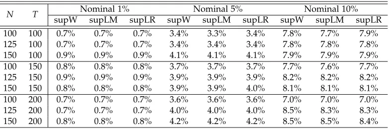
Remark 7.1 The powers of the supW, supLM and supLR tests can be studied in the same way under the local alternative̟⋆ = ̟∗+µ(t/T)/√NT, where ̟∗ = (ρ∗,β∗′a )′ with β∗a
is the coefficients of the exogenous regressors that are suspected to experience a struc-tural change, and µ(·)is a bounded real-valued function on[0, 1], which satisfies some regularity conditions. For more details, see Assumption 1-LP and the related discussions in Andrews (1993). We will not pursuit this work for the sake of space.
Remark 7.2 The critical values for the supW, supLM and supLR tests are given in An-drews (2003) and Estrella (2003). The critical values depend on the column dimension of Xt(i.e., the value q) and the chosen interval[γL,γU]. As γL decreases to zero and γU
increases to one, the critical values would diverge to infinity, a result which is shown in Corollary 1 of Andrews (1993). Many studies recommend that the interval is chosen to be [0.15, 0.85], e.g., Andrews (1993). We will adopt this interval in our simulations investigation. Given this interval, according to Estrella (2003), the critical values for 10%, 5% and 1% significance levels are 10.14, 11,87 and 15.69 when p = 1, and 12.46, 14.31 and 18.36 whenp=2.
Remark 7.3 The supW, supLM and supLR statistics in the dynamic model can be con-structed similarly as those in the static model. The only caveat is that these statistics should be computed through the bias-corrected MLE, instead of the original one, to re-move the effect of bias. The analyses on the three statistics in the dynamic model are similar as in the static model, by treatingYt−1 as a part ofZt. Under the condition that
N/T3 →0, we can show that these three statistics have the same limiting distribution as in Corollary 7.1.
8
Simulations
We run Monte Carlo simulations to investigate the finite sample performance of the ML estimators in this section.
8.1 Static spatial panel data models
The data are generated according to
Yt =α+ρ∗WNYt+̺∗WNYt✶(t≤[Tγ∗]) +Xt1β∗1+Xt2β∗2+Xt1✶(t ≤[Tγ∗])δ∗+Vt,
with (ρ∗,̺∗,β∗
1,β∗2,δ∗,γ∗,σ∗2) = (0.4,−0.1, 2, 1,−1, 0.25, 0.36). Our data generating
the other does not. The spatial weights matrices used in simulations are “qahead and qbehind” spatial weights matrix as in Kelejian and Prucha (1999), which is obtained as follows: all the units are arranged in a circle and each unit is affected only by thequnits immediately before it and immediately after it with equal weight. Following Kelejian and Prucha (1999), we normalize the spatial weights matrix by letting the sum of each row equal to 1. In our simulations, we consider “3 ahead and 3 behind”.
All the elements of the exogenous regressors Xt1,Xt2 and the intercept αare drawn
independently from N(0, 1). The disturbance vit, the ith element ofVt, is 0.6 times of a
normalizedχ2(2), i.e., [χ2(2)−2]/2. OnceX
t1,Xt2,αandVt are generated, we calculate
Yt by
Yt=
h
IN−ρ∗WN−̺∗WN✶(t ≤[Tγ∗])
i−1h
α+Xt1β∗1+Xt2β∗2+Xt1✶(t≤ [Tγ∗])δ∗+Vt
i
.
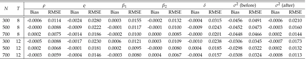
Throughout this section, we use bias and root mean square error (RMSE) as the mea-sures of the performance of the ML estimators. To investigate the estimation accuracy of asymptotic variances, we calculate the empirical sizes of thet-statistic for 5% nominal level. Table 1 presents the simulation results under the combinations of N = 50, 75, 100 and T = 50, 75, 100, which are obtained by 1000 repetitions. In this section, we do not evaluate the performance of ˆγ, partly because the bias and RMSE are not appropriate measures with respect to ˆγ, and partly because the performance of ˆγis implicitly shown in the performance of the ML estimators for the other parameters. From Table 1, we have following findings. First, the ML estimators are consistent. As N and T tends to large, the RMSE decrease stably. Second, the ML estimators for ρ,̺,β andδ are unbi-ased. In all the sample sizes, the biases of these ML estimators are very small in terms of both absolute values and relative values, where the relative value is defined by the ratio of bias and RMSE. Third, the ML estimator forσ2 is biased, and the bias is loosely related with N and closely related with T. Consider the case of T = 50, the biases are
−0.0073,−0.0077 and−0.0074 for N =50, 75 and 100. Obviously, the increase of N has no effect on the bias, but when T grows larger, the bias decrease dramatically. This is consistent with our theoretical result in Theorem 4.2. Table 2 presents the results under the combination of N = 300, 500, 700 andT = 8, 12. The results are similar as those in Table. So we do not repeat the analysis.
Table 1: The performance of the MLE with moderate largeTin the static model
N T ρ ̺ β1 β2 δ σ2(before) σ2(after) Bias RMSE Bias RMSE Bias RMSE Bias RMSE Bias RMSE Bias RMSE Bias RMSE
30 50 -0.0008 0.0101 -0.0007 0.0273 0.0004 0.0140 0.0005 0.0122 0.0003 0.0290 -0.0073 0.0213 -0.0001 0.0204 75 50 0.0000 0.0085 -0.0018 0.0231 0.0002 0.0121 -0.0001 0.0100 0.0003 0.0247 -0.0077 0.0179 -0.0005 0.0165 100 50 0.0000 0.0074 -0.0005 0.0202 -0.0003 0.0097 0.0003 0.0083 0.0015 0.0204 -0.0074 0.0160 -0.0002 0.0144 50 75 -0.0006 0.0084 -0.0007 0.0222 0.0003 0.0116 -0.0001 0.0095 0.0001 0.0237 -0.0047 0.0165 0.0001 0.0161 75 75 -0.0001 0.0069 -0.0009 0.0189 -0.0000 0.0095 0.0002 0.0078 -0.0005 0.0193 -0.0056 0.0145 -0.0008 0.0136 100 75 0.0001 0.0057 -0.0003 0.0156 -0.0004 0.0080 -0.0000 0.0070 -0.0000 0.0162 -0.0051 0.0122 -0.0003 0.0112 50 100 -0.0002 0.0073 0.0002 0.0195 0.0002 0.0101 0.0002 0.0087 -0.0009 0.0196 -0.0032 0.0147 0.0004 0.0145 75 100 -0.0001 0.0060 -0.0007 0.0154 -0.0002 0.0081 -0.0004 0.0071 -0.0001 0.0164 -0.0040 0.0124 -0.0004 0.0119 100 100 -0.0002 0.0052 0.0000 0.0136 -0.0001 0.0068 -0.0002 0.0058 -0.0001 0.0140 -0.0037 0.0105 -0.0001 0.0099
Table 2: The performance of the MLE with smallTin the static model
N T ρ ̺ β1 β2 δ σ
2(before) σ2(after)
Bias RMSE Bias RMSE Bias RMSE Bias RMSE Bias RMSE Bias RMSE Bias RMSE
300 8 -0.0006 0.0114 -0.0024 0.0280 0.0003 0.0155 -0.0002 0.0132 -0.0004 0.0315 -0.0456 0.0491 -0.0006 0.0210 500 8 -0.0000 0.0088 -0.0009 0.0222 -0.0001 0.0117 -0.0001 0.0100 -0.0009 0.0243 -0.0452 0.0473 -0.0003 0.0160 700 8 0.0002 0.0075 -0.0014 0.0186 -0.0002 0.0100 0.0000 0.0085 -0.0000 0.0201 -0.0448 0.0466 0.0002 0.0144 300 12 -0.0005 0.0088 -0.0017 0.0230 0.0006 0.0121 0.0003 0.0109 -0.0010 0.0238 -0.0306 0.0345 -0.0007 0.0173 500 12 0.0002 0.0068 -0.0001 0.0181 0.0002 0.0095 -0.0000 0.0080 0.0004 0.0185 -0.0298 0.0322 0.0002 0.0132 700 12 -0.0003 0.0059 -0.0004 0.0146 -0.0003 0.0080 0.0004 0.0067 -0.0004 0.0157 -0.0308 0.0324 -0.0008 0.0113
Note:σ2(before) andσ2(after) denote the estimators before and after the bias correction, respectively.
[image:23.792.107.688.344.457.2]Table 3: The empirical sizes oft-test under nominal 5% significance level in moderate large-T setup
N T ρ ̺ β1 β2 δ σ
2
before after
50 50 4.6% 5.3% 5.1% 5.0% 5.1% 10.1% 6.8%
75 50 5.4% 5.6% 6.1% 6.2% 6.0% 9.7% 6.1%
100 50 5.8% 5.9% 5.3% 4.2% 5.1% 10.2% 4.8%
50 75 5.2% 4.4% 4.6% 4.4% 5.7% 5.8% 4.9%
75 75 5.3% 5.5% 5.7% 4.3% 5.5% 9.6% 6.4%
100 75 3.8% 5.0% 4.3% 5.8% 5.1% 7.9% 4.0%
50 100 5.4% 5.2% 5.4% 5.7% 5.1% 6.0% 4.7%
75 100 4.9% 4.1% 5.0% 5.5% 5.2% 6.8% 5.5%
100 100 5.3% 5.4% 4.1% 4.4% 5.1% 7.0% 4.7%
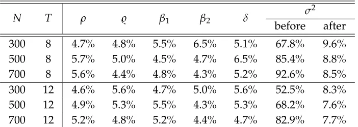
Table 4: The empirical sizes of t-test under nominal 5% significance level in small-T setup
N T ρ ̺ β1 β2 δ σ
2
before after
300 8 4.7% 4.8% 5.5% 6.5% 5.1% 67.8% 9.6%
500 8 5.7% 5.0% 4.5% 4.7% 6.5% 85.4% 8.8%
700 8 5.6% 4.4% 4.8% 4.3% 5.2% 92.6% 8.5%
300 12 4.6% 5.6% 4.7% 5.0% 5.6% 52.5% 8.3% 500 12 4.9% 5.3% 5.5% 4.3% 5.3% 68.2% 7.6% 700 12 5.2% 4.8% 5.2% 4.4% 4.7% 82.9% 7.7%
ˆ
σ2, which suffers a mild size distortion under moderate largeT and a severe size
distor-tion under fixedT. But after conducting bias correction, the performance has been much improved. Overall, the performance of the MLE after bias correction are satisfactory.
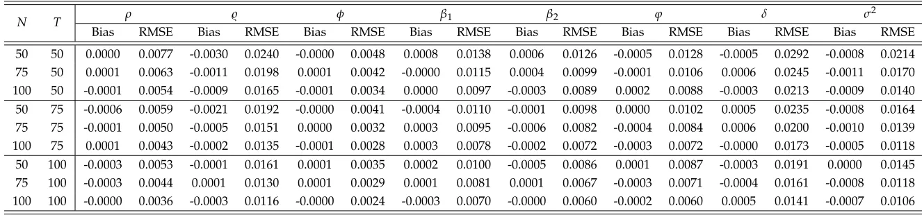
8.2 Dynamic spatial panel data models
We next examine the performance of the ML estimators in the dynamic model. The data are generated according to
Yt =α+ρ∗WNYt+̺∗WNYt✶(t≤[Tγ∗]) +Yt−1φ∗+Xt1β∗1+Xt2β∗2 +Yt−1✶(t ≤[Tγ∗])ϕ∗+Xt1✶(t≤ [Tγ∗])δ∗+Vt,
with(ρ∗,̺∗,φ∗,β∗1,β∗2,ϕ∗,δ∗,γ∗,σ∗2) = (0.4,−0.1, 0.5, 2, 1,−0.2,−1, 0.25, 0.36). The
inter-ceptα∗, the exogenous regressorsXt1andXt2and the disturbanceVtare generated by the
same way in the static model. The data of dependent variable is calculated recursively by
Yt =
h
IN−ρ∗WN−̺∗WN✶(t≤[T