Semiparametric Estimation and Testing of Smooth Coefficient Spatial Autoregressive Models

Munich Personal RePEc Archive

Semiparametric Estimation and Testing

of Smooth Coefficient Spatial

Autoregressive Models

Malikov, Emir and Sun, Yiguo

Auburn University, University of Guelph

February 2017

Online at

https://mpra.ub.uni-muenchen.de/77253/

Semiparametric Estimation and Testing of Smooth

Coefficient Spatial Autoregressive Models

∗

Emir Malikov1 Yiguo Sun2

1_{Department of Agricultural Economics & Rur. Soc., Auburn University, Auburn, AL} 2

Department of Economics and Finance, University of Guelph, ON

First Draft: December 15, 2014 This Draft: February 25, 2017

Abstract

This paper considers a flexible semiparametric spatial autoregressive (mixed-regressive) model in which unknown coefficients are permitted to be nonparametric functions of some contex-tual variables to allow for potential nonlinearities and parameter heterogeneity in the spatial relationship. Unlike other semiparametric spatial dependence models, ours permits the spatial autoregressive parameter to meaningfully vary across units and thus allows the identification of a neighborhood-specific spatial dependence measure conditional on the vector of contextual variables. We propose several (locally) nonparametric GMM estimators for our model. The developed two-stage estimators incorporate both the linear and quadratic orthogonality condi-tions and are capable of accommodating a variety of data generating processes, including the instance of a pure spatially autoregressive semiparametric model with no relevant regressors as well as multiple partially linear specifications. All proposed estimators are shown to be consis-tent and asymptotically normal. We also contribute to the literature by putting forward two test statistics to test for parameter constancy in our model. Both tests are consistent.

Keywords: Consistent Test, Constrained Estimation, Local Linear Fitting, Nonparametric GMM, Partially Linear, Quadratic Moments, SAR, Spatial Lag

JEL Classification: C13, C14, C21

∗_{Email: [email protected] (Malikov), [email protected] (Sun).}

1

Introduction

While spatial econometric methods have solidly become part of a standard methodological toolkit of applied researchers in many fields of economics that deal with spatial data which include appli-cations such as land use, hedonic pricing or cross-country growth studies, most empirical work has confined its analysis to linear spatial models only. However, to paraphrase Paelinck & Klaassen (1979), econometric relations in space result more often than not in highly nonlinear specifications (as cited in van Gastel & Paelinck, 1995). For instance, allowing for nonlinearities in the hedonic house price function is often argued to be crucial in order to obtain realistic marginal valuations of housing attributes (e.g., see Parmeter, Henderson & Kumbhakar, 2007). Taking such potential nonlinearities in spatial models for granted is likely to lead to inconsistent parameter estimates and thus misleading conclusions.

This paper proposes a semiparametric method to handling nonlinearity (and parameter hetero-geneity) in models of spatial dependence. We extend a particular class of semiparametric models in which parameters of a linear regression are permitted to be unspecified smooth functions of some contextual variables (Hastie & Tibshirani, 1993; Cai, Fan & Li, 2000; Li, Huang, Li & Fu, 2002) to the case of data with spatial dependence. Specifically, we generalize a popular parametric spatial autoregressive mixed-regressive model by allowing its coefficients, including the spatial autoregres-sive parameter, to be nonparametric functions of unknown form [for concreteness, see eq. (2.1)].

While our “smooth coefficient” spatial autoregressive model closely relates to the family of partially linear semiparametric spatial models recently proposed in the literature (Su & Jin, 2010; Su, 2012; Zhang, 2013; Sun, Hongjia, Zhang & Lu, 2014), its distinct feature is that it permits the spatial autoregressive parameter to meaningfully vary across units. The latter may be highly desirable from a practitioner’s point of view since it allows the identification of a neighborhood-specific spatial dependence measure conditional on the vector of contextual variables. For instance, when a spatial autoregressive model is game-theoretically rationalized as a “response function”, our model empowers a researcher to estimate heterogeneous “reaction” parameters that can vary with some environmental control factors. Some potential applications of our model, for instance, include the estimation of growth models that explicitly account for technological interdependence between countries in the presence of spillover effects. Such technological interdependence is usually formulated in the form of spatial externalities (e.g., see Ertur & Koch, 2007). However, the inten-sity of knowledge spillovers is naturally expected to greatly depend on institutional and cultural compatibility of neighboring countries (Kelejian, Murrell & Shepotylo, 2013). Our smooth coef-ficient spatial autoregressive model presents a practical, easy-to-implement way to allow for such indirect effects of institutions on the degree of spatial dependence in the cross-country conditional convergence regressions.

we therefore abstract from the issue concerning the correct specification of spatial weights.1 We propose several (locally) nonparametric Generalized Method of Moments (GMM) estimators for our model. The developed estimators incorporate both the linear and quadratic orthogonality conditions and are capable of accommodating a variety of data generating processes, including the instance of a pure spatially autoregressive semiparametric model with no relevant regressors as well as multiple partially linear specifications. To this end, we contribute to the literature on four fronts. First, our paper is the first (to the best of our knowledge) attempt in the nonparametric estimation literature to make use of local quadratic orthogonality conditions, which are necessary for the IV identification of spatially autoregressive models in the case when all explanatory covariates are irrelevant in predicting the outcome variable (see Lee, 2007). Second, we propose a two-stage estimation procedure whereby we first obtain an initial estimator of unknown parameter functions using feasible, but likely not so strong, instruments which we then use for the construction of more natural instruments suggested by the model’s reduced form. Again, to our knowledge, no prior attempt has been made in the nonparametric econometrics literature to study such a class of estimators which themselves are based on the estimated instruments. Third, we also consider two special cases of our model by allowing some of its parameter functions to be constant thus resulting in a partially linear specification. Our proposed estimators present an alternative to those by Su (2012) and Zhang (2013) who study a similar class of partially linear spatial models. Unlike their estimators, ours however preserves its consistency property if the true model is a pure spatial autoregression. Fourth, we discuss ways of ensuring that the estimated model satisfies the non-singularity condition needed to rule out unstable Nash equilibria. In the instance of a mixed-regressive model, we impose this non-singularity restriction via the “tilting” procedure `a la Hall & Huang (2001) whose theoretical results we generalize to the case of GMM estimators in the presence of endogenous regressors. Under fairly mild regularity conditions, we show that all our proposed estimators are consistent and asymptotically normal.

Further, we contribute to the literature by putting forward two test statistics to test for pa-rameter constancy in our model. These model specification tests allow us to discriminate between a standard linear spatial autoregressive and our semiparametric models. The first consistent test utilizes a popular residual-based specification test technique which we extend to spatial data with cross-sectional dependence.2 Given the well-known poor performance of nonparametric residual-based tests in finite samples, we also suggest a (wild) bootstrap procedure for it which we show to be asymptotically valid in approximating the null distribution of our test statistic regardless of whether the null hypothesis holds true or not. However, our residual-based test is impractical when the spatial model has no regressors. We therefore propose an alternative consistent test statistic `a la Henderson, Carroll & Li (2008) which provides a vehicle for testing for parameter constancy in our model even when the model is a pure spatial autoregression.

We investigate the finite sample performance of the proposed estimators and test statistics in a small set of Monte Carlo experiments. The results are encouraging and show that all estimators and tests perform well in finite samples with considerable improvements as the sample size increases. Overall, simulation experiments lend support to our asymptotic results. To showcase our method-ology, we then apply it to estimate a spatial hedonic price function using the well-known Harrison & Rubenfeld’s house price data from Gilley & Pace (1996), where we let unknown parameter

func-1

Furthermore, theoretical basis for the widely-believed sensitivity of the estimates to the choice of spatial weights remains rather unclear, as recently argued by LeSage & Pace (2014).

2

tions to vary with the NOx concentration in the air. We find that spatial dependence between house prices is statistically significant only at higher values of the NOxconcentration in the air and that the degree of this spatial dependence, on average, increases as the air quality declines. This finding suggests that locational similarity may matter little for house valuations in pollution-free localities.

The rest of the paper proceeds as follows. Section 2 outlines the model. We present our estimators in Section 3, where we also provide their large-sample statistical properties. In Section 4, we consider two different types of partially linear spatial autoregressive models. Section 5 discusses specification tests for parameter constancy. The results of Monte Carlo simulations are described in Section 6. Section 7 concludes.

Throughout the paper, we use M to denote a generic finite constant that can take different values at different appearances and vec_{A_}stacks columns of ann_×mmatrixAinto an (nm)_×1 vector. Lastly, tr_{A_} refers to the trace of a square matrix A.

2

Semiparametric Spatial Autoregressive Model

Consider a semiparametric generalization of the conventional (linear) spatial autoregressive mixed-regressive model, where the coefficients are now permitted to be unknown smooth functions of some relevant exogenous variables, i.e.,

yi=ρ(zi)

X

j6=i

wijyj+x′iβ(zi) +ui ∀ i= 1, . . . , n, (2.1)

where yi is the (scalar) outcome variable of interest; xi and zi are p ×1 and q ×1 vectors of exogenous covariates, respectively, and xi can contain a constant 1; wij is the (i, j)-th element of a given n_×n non-stochastic spatial weighting matrix W such that wii = 0 for all i. Further,

β(zi) is a conformable vector of unknown slope parameter functions of zi, and ρ(zi) is an un-known (scalar) spatial lag parameter function of zi. The random disturbance ui is identically and independently distributed over i conditional on (xi,zi) with zero mean and finite variance, i.e., ui|xi,zi ∼ i.i.d. (0, σu2).

We proceed by rewriting model (2.1) in the matrix form as

y=ρ(Z)Wy+ mtx_{X,β(Z)_}+u, (2.2)

where y = (y1, . . . , yn)′ and u = (u1, . . . , un)′ are n×1 vectors; ρ(Z) ≡diag{ρ(z1), . . . , ρ(zn)} is ann_×ndiagonal matrix of spatial autoregressive parameter functions; and mtx_{·}is the operator that stacks up x′_iβ(zi) into an n×1 vector with thei subscript matching those ofy,u and ρ(Z). Also,X=x1 . . . xn′ and Z=z1 . . . zn′ are n×p and n×q data matrices, respectively. To facilitate the economic interpretation of ρ(zi) as the “reaction” parameter (and to rule out unstable Nash equilibria), we assume the following condition forρ(_·) to ensure the non-singularity of In−ρ(Z)W:3

max

1≤i≤n|λi{ρ(Z)W}|<1, (2.3) whereλi{A} is the ith eigenvalue of an n×nmatrixA.

3

Model (2.1) nests a standard smooth coefficient model with strictly exogenous covariates (Cai et al., 2000; Li et al., 2002) as a special case when ρ(zi) = 0 for all i, which implies no spatial interaction in the outcome variable yi. In many applications, it is however imperative to allow for potential spatial dependence in the data. For instance, house prices are widely believed to be spatially autoregressive because residential property values tend to reflect shared local ameni-ties as well as observed and unobserved neighborhood characteristics. While these characteristics can be partly controlled for using locality fixed effects, such an approach may be quite unsat-isfactory since it does not let characteristics of neighboring houses affect the price of a given house (Anselin & Lozano-Gracia, 2009). However, by including the spatial lag in a house pricing function, we are able to accommodate such cross-neighbor effects as can be seen from the follow-ing expansion of the reduced form of equation (2.2) under the non-sfollow-ingularity condition in (2.3):

E_{[y|X,Z] = [In−ρ(Z)W]}−1_{mtx{X,β(Z)}=}

∞ X

s=0

ρ(Z)Wsmtx_{X,β(Z)_}. (2.4)

From (2.4), it is evident that the conditional mean of yi depends not only on its ownxi and zi but also on its neighbors’xj andzj forj6=i. Perhaps more importantly, house prices are likely to be spatially autoregressive because the very process of property valuation at its core relies on sale price information for comparable houses in the local neighborhood that real estate agents base their appraisals on. The latter is known as the “sales comparison approach” to a real estate appraisal which can systematically influence equilibrium prices in the housing market, especially if property owners have limited information about the market (see the reference in Small & Steimetz, 2012). Our model will be able to accommodate this spatial dependence in house prices while also allowing for nonlinearities and parameter heterogeneity in the house valuation function.

Studies of institutional change provide another example of applications where it is crucial to explicitly model spatial dependence in the data. Existing theoretical and empirical work indicate that institutional development in one country affects that of its neighbors (Mukand & Rodrik, 2005), where the institutional diffusion may be driven, say, by lobbying of multinational corporations for the harmonization of the commercial law across countries, requirements for members of a trade pact to standardize regulations or even military conflicts (see Kelejian et al., 2013). The semiparametric model we propose is equipped to examine such institutional diffusions across space while also allowing for nonlinearities and heterogeneity in institutional spillovers.

Lastly, in the instance when ρ(zi) is a non-zero constant for all i, our model nests a partially linear smooth coefficient spatial autoregressive model as a special case (see Sun et al., 2014).

Remark 1 The differentiation between the two sets of covariates, xi and zi, is a practitioner’s prerogative which is likely to change from one empirical application to another. The assignment of relevant regressors into either of the two sets of variables may be done on the basis of practical convenience or, better yet, economic theory suggesting the direct (X) and indirect, contextual (Z) determinants of the spatially correlated outcome variable. From the theory’s point of view however, our results do not require the variables inxi to be different from or unrelated to those inzi.

3

Nonparametric GMM Estimator

We propose to estimate the unknown coefficient functions [ρ(zi),β(zi)′]′ in (2.1) by a local linear regression approach. First, we rewrite equation (2.1) in a compact form as follows:

where mi ≡hP_j6=iwijyj

,x′_ii′ and γ(zi) ≡ [ρ(zi),β(zi)′]′ are (p+ 1)×1 vectors. Model (3.1) seemingly takes the form of the standard semiparametric smooth coefficient model subject to en-dogeneity in one of the covariates, namely, the spatial lag termP_j6=iwijyj. We estimate the above model using the (locally) nonparametric GMM estimator along the lines of Cai & Li (2008) subject to the non-singularity condition (2.3).

Under the assumption that smooth parameter functions are twice continuously differentiable in the neighborhood of z, each element inγ(_·) can then be approximated by its first-order Taylor expansion aroundz, i.e.,γs(zi)≈γs(z) +∇γs(z)′(zi−z) at pointzi close toz fors= 1, . . . , p+ 1, where_∇γ_s(z)_≡[∂γs(z)/∂z1, . . . , ∂γs(z)/∂zq]′ is aq×1 vector of the first-order derivative ofγs(·). Therefore, for zi close toz, we can approximate (3.1) by

yi ≈m′iθ(z)Zi(z) +ui= [Zi(z)⊗mi]′vec{θ(z)}+ui ∀ i= 1, . . . , n, (3.2) where _Zi(z) ≡ [1,(zi−z)′H−1]′ is a (q+ 1)×1 vector with H = diag{h1, . . . , hq} being a q×q diagonal bandwidth matrix, and

θ(z)_≡

  

γ1(z) ∇γ1(z)′H ..

. ...

γp+1(z) ∇γp+1(z)′H

  

denotes a (p+ 1)_×(q+ 1) parameter matrix.

Before introducing our estimator, we first take a closer look at the spatial lag term. Denoting Sn(Z)≡[In−ρ(Z)W]−1 andGn(Z)≡WSn(Z), we have the reduced form of our model in (2.2):

y=Sn(Z) (mtx{X,β(Z)}+u),

from where it is evident that the spatial lag termWy=Gn(Z) [mtx{X,β(Z)}+u] is endogenous because E_(Gn(Z)u)′_{u =σu}2E_{[tr{Gn(Z)}]6= 0 in general. Now, let Pn be some n×n matrix}

satisfying E_(Pnu)′_{u= 0. We then can rewrite Wy as follows: Wy =Gn(Z) mtx{X,β(Z)}+}

Pnu + [Gn(Z)−Pn]u, where both Gn(Z) mtx{X,β(Z)} and Pnu are uncorrelated with u. This observation suggests that Gn(Z) mtx{X,β(Z)} and Pnu can be reasonable valid instru-ments for Wy. There are multiple choices for the matrix Pn with a zero-trace Pn = Gn(Z)− n−1tr_{Gn(Z)}Inand a zero-diagonalPn=Gn(Z)−diag{Gn(Z)}being among the most popular specifications in the parametric spatial regression literature (e.g., Kelejian & Prucha, 1999; Lee, 2007). However, note that neitherGn(Z) mtx{X,β(Z)} norPnu are feasible instruments due to the presence of unknown smooth coefficientsρ(Z) andβ(Z) inGn(Z). In this paper, we therefore propose to first obtain an initial consistent estimator of unknown parameter functions using feasible instruments (in Section 3.1) and then to construct a second-stage estimator (in Section 3.2) which instruments for the endogenous spatial lag withGn(Z) mtx{X,β(Z)} andPnu constructed using the initial first-stage consistent estimator of ρ(_·) andβ(_·). In what follows, we describe these two proposed estimators.

3.1 First-Stage Estimator

The expansion in (2.4) suggests thatWX,WZ,W2X,W2Z,. . . with linearly dependent columns removed can be valid instruments for the endogenous spatial lag term Wy. Also note that both matrices Pn,l = Wl −n−1trWl In and Pn,l = Wl−diagWl for l = 1,2, . . . satisfy

E_(Pn,lu)′_{u= 0. We thus have identified feasible instruments which can be employed to obtain}

Define ann_×dmatrix of instrumentsQn= [Q1n,X]≡Qn,1 . . . Qn,n′, whereQ1ncontains linearly independent instruments taken from WX,WZ,W2X,W2Z, . . . . We then obtain the following kernel-weighted (local) orthogonal conditions:

Eh_Q(z)′_{KH(z)y−M(z)vec{θ(z)}}i_{≈0d (3.3)}

and

E_{y−M(z)vec{θ(z)}}′_{Pn,lKH(z)y−M(z)vec{θ(z)}≈0 ∀ l= 1,2, . . . , m (3.4)}

for a finite integer m, where M(z) = _Z1(z)⊗m1 . . . Zn(z)⊗mn′ is an n×[(p+ 1)(q+ 1)] data matrix; Q(z) = _Z1(z)⊗Qn,1 . . . Zn(z)⊗Qn,n′ is an n×[d(q+ 1)] instrument matrix; KH(z) = diag{KH(z1, z), . . . ,KH(zn, z)} is an n×n diagonal matrix of kernel weights with

KH(zi, z) =K H−1(zi−z) being a product kernel. Denoting

gn(θ) =

       

y₋M(z)vec_{θ_}′Pn,1KH(z)

y₋M(z)vec_{θ_}

.. .

y₋M(z)vec_{θ_}′Pn,mKH(z)

y₋M(z)vec_{θ_}

Q(z)′KH(z)

y₋M(z)vec_{θ_}

       

(3.5)

for a (p+ 1)_×(q+ 1) vector θ, we construct our initial first-stage nonparametric GMM estimator: vecnθb(z)o= arg min

θ(z)

gn(θ(z))′gn(θ(z)). (3.6)

Below, we list assumptions used to derive the limiting distribution of our proposed estimator.

Assumption 1 _{(xi,zi, ui)} is i.i.d. over index i, yi is generated according to (2.1) satisfying (2.3). Also, E_kxik2(2+δ1)

< M and Eh_kzik4(2+δ1)i

< M for someδ1 >0.

(i) E_{[ui|xi =x,zi =z] = 0,} E_u2

i|xi=x,zi=z= σu2 >0 and E

h |ui|4+δ

xi=x,zi=z

i

< M for any x_∈Rp _andz∈Rq _{and some δ >0;}

(ii) There exists a positive integer N such that both W and [In−ρ(Z)W]−1 have finite row-and column-sum matrix norms for all n > N;

(iii) Pn,l is an n×n matrix with finite row- and column-sum matrix norms for all n > N and tr_{Pn,l} = 0 for alll = 1, . . . , m, where m ≥ 1 is a finite positive integer. And, the n×d instrument matrixQnhas a full rank d≥p+ 1.

Here, the row- and column-sum matrix norms of some n_×nmatrixA are respectively defined as_kA_krow = max1≤i≤nPnj=1|aij|and kAkcolumn = max1≤j≤nPni=1|aij|. Assuming ui has a finite (4 +δ)th-order conditional moment in Assumption 1(i) is necessary to apply the central limit theorem derived by Kelejian & Prucha (2001).

Assumption 2 (i)ρ(z),β(z),f(z) andE_[Qn,im′

i|zi =z] are all twice continuously differentiable in a neighborhood ofz, wheref(z)>0 is the probability density function ofzi evaluated at point z; (ii) E_kQn,ik2+δ1

|zi =z

Assumption 3 The kernel functionk(v) is a symmetric probability density function with a com-pact support [₋1,1]. Also, we define µi,j(k) = Rki(v)vjdv and R2(K) = R K2(v)dv, where

K(v) =Qq_j=1k(vj) andv= [v1, . . . , vq]′.

Assumption 4 As n _{→ ∞}, _kH_{k →} 0, n_|H_{| → ∞}, and limn→∞n|H| kHk4 = c0 > 0, a finite constant, where _|H_|=Qq_j=1hj and kHk2=Pqj=1h2j.

Theorem 1 Under Assumptions 1–4, and if κ_{B(H, z) is nonsingular at an interior point z, we}

have

p

n_|H_|

b

γ(z)₋γ(z)₋µ1,2(k)

2 Bias(H, z)

d

→ N_{0p+1, f}−1_{(z)R2(K) plim}

n→∞

κ_{B(H, z)}−1_{Ω(z) plim}

n→∞

κ_{B(H, z)}−1_,

where Bias(H, z) = Sp+1κB(H, z)−1κA(H, z)′ = Op

kH_k2, Sp+1 equals the first p+ 1 rows of the identity matrix I[(p+1)(q+1)], and κA(H, z), κB(H, z), and Ω(z) are respectively defined in Lemmas 1, 2 and 3 in Appendix A.

Theorem 1 states that the local linear estimator of the varying coefficients ρ(z) and β(z) has the conventional bias term of orderOp

kH_k2and asymptotic variance of orderOp

(n_|H_|)−1/2.

Remark 2 As discussed in Lemma 2, κ_{B(H, z) can be singular ifX is irrelevant in predicting y}

or β(z) = 0p holds true over its domain. However, this problem occurs only to the local linear regression approach and not to the local constant approach. Thus, the estimator derived from the nonparametric GMM via a local constant fitting doesnot suffer from the singularity problem even ifX is irrelevant fory.

Next, notice that, since θb(z) in (3.6) does not have an analytic formula due to the use of the

quadratic moment (3.4), the computation of our estimator can be significantly slow for relatively large samples. However, if one is reasonably confident that β(z) is a non-zero vector over at least one non-empty subset, we are able to construct an alternative consistent estimator of γ(z) which has a simple closed-form formula and hence is fast to compute. This alternative estimator uses the

linear local orthogonal condition in (3.3) only.4

Specifically, we are interested in minimizing the following (local) objective function:

min θ(z)

h

Q(z)′KH(z)

y₋M(z)vec_{θ(z)_}i′Q(z)′KH(z)

y₋M(z)vec_{θ(z)_}, (3.7)

which yields

vecnbθ(z)o=hM(z)′ΞH(z)M(z)

i−1

M(z)′ΞH(z)y, (3.8)

where ΞH(z) ≡KH(z)′Q(z)Q(z)′KH(z). Following the proof of Theorem 1, we obtain the limit result for vecnbθ(z)oas follows.

4

Note that Qn is not a valid instrument matrix if X and Zare both irrelevant in predicting y, which occurs if

β(z) = 0p and ρ(z) = ρ0 over their domains and our model (2.1) becomes a pure spatial autoregressiony_i =

ρ0P

Corollary 2 Under Assumptions 1–4 and assuming E1(z)′E1(z) is non-singular, at an interior pointz, we have

p

n_|H_|

b

γ(z)₋γ(z)₋µ1,2(k)

2 Bias(H, z)

d

→ N_0p+1, σ

2 u

f(z)R2(K)Σ(z)

,

where Bias(H, z) = [E1(z)′E1(z)]−1E1(z)′E2(H, z)′ =O

kH_k2,

Σ(z) =E1(z)′E1(z)−1E1(z)′E3(z)E1(z) E′1(z)E1(z)−1

andE1(z),E2(H, z) andE3(z) are respectively defined in (A.8), (A.9) and (A.24) in Appendix A.

3.2 Second-Stage Estimator

Having obtained the initial estimator of unknown parameter functions ρ(_·) and β(_·) in (3.6), we can now construct the feasible versions of our originally desired instruments, namely, Qb1n =

b

Gn(Z) mtx

n

X,βb(Z)oand, e.g., the zero-tracePbn=Gbn(Z)−n−1tr

n b

Gn(Z)

o

In, whereGbn(Z) =

W[In−bρ(Z)W]−1. With this, we derive our second-stage nonparametric GMM estimator:

vecneθ(z)o= arg min θ(z)

gn(θ(z))′gn(θ(z)) , (3.9)

where the moment function is defined as

gn(θ) =

 

y₋M(z)vec_{θ_}′PbnKH0(z)

y₋M(z)vec_{θ_}

b

Q(z)′KH0(z)

y₋M(z)vec_{θ_}



, (3.10)

H0 is the newq×q diagonal bandwidth matrix; andM(z), Qb(z) and vec{θ}are as defined earlier except forQb(z) being constructed usingQb1n in place ofQ1n.

Asymptotic results for our second-stage estimator require the following additional assumptions.

Assumption 5 sup_z∈Szkbγ(z)₋γ(z)_k=Op

kH_k2+plnn/(n_|H_|).

Assumption 6 (i)_kH_{k →}0,_kH0k →0 ,n|H| → ∞,n|H0| → ∞, andn|H0| kH0k4=O(1); (ii)

kH_k4/_|H0| kH0k2

→0,n_|H_{| |}H0| kH0k2/lnn→ ∞, andn

p

|H_{| |}H0| kH0k3/lnn→ ∞.

Assumption 5 strengthens the pointwise consistency result for γb(z) to a uniform convergence result over its domain _Sz. This is a reasonable result to be expected if one assumes that Sz is a compact subset of Rq _{and v}j_{k(v) satisfies Lipschitz condition for 0 ≤ j ≤ 3 by closely following}

more than one continuous variable, one needs to apply a higher-order local polynomial approach in the first-stage estimation to ensure the optimal convergence rate in the second-stage estimation. For instance, if we apply the local rth-order polynomial approach with an odd integer r _≥ 1,

kH_k4/_|H0| kH0k2

=o(1) in Assumption 6(ii) will be replaced by_kH_k2(r+1)/_|H0| kH0k2

= o(1). Withα0 = 1/(4 +q), we haveα0(2 +q)/[2 (r+ 1)]< α <[1−(q+ 3)α0] 2/q which implies that q < √4r+ 5₋1. So, if q = 2, r > 1 is required, and hence we can apply the local cubic polynomial approach in the first-stage estimation in that instance.

Theorem 3 Under Assumptions 1–3, 5 and 6, at an interior pointz, we have

p

n_|H0|

e

γ(z)₋γ(z)₋ µ1,2(k)

2 Bias(H0, z)

d

→ N_{0p+1, f}−1_{(z) plim}

n→∞

κ_B(H0, z)−1Ω(z) plim

n→∞

κ_{B(H0, z)}−1_,

where Bias(H0, z) = Sp+1κB(H0, z)−1κA(H0, z)′, and κA(H0, z), κB(H0, z) and Ω(z) are re-spectively defined in Lemmas 4, 5 and 6 in Appendix A.

Theorem 3 states that the second-stage estimator is consistent and has an asymptotic normal distribution at the usual nonparametric convergence rate with the proper order of a local polyno-mial estimation approach. Intuitively, the second-stage estimator is expected to be asymptotically more efficient than its first-stage counterpart because the instruments employed in the first-stage estimation have lower predictive power forWythan those used in the second stage. This intuition is confirmed by our Monte Carlo simulations in Section 6.1. However, we are unable to analytically verify this result since both asymptotic variances in Theorems 1 and 3 take complex forms.

Remark 3 The consistency and asymptotic normality results for the second-stage estimator con-tinue to hold if we use the zero-diagonal Pbn =Gbn(Z)−diag

n b

Gn(Z)

o

in (3.10). Naturally, the definition ofκ_{A(H0, z),}κ_{B(H0, z) andΩ(z) referenced in Theorem 3 will change accordingly.}

3.3 Non-Singularity Constraint

Until now, we have proceeded with the estimation of (2.1) as if it were a standard smooth coefficient model subject to endogeneity in one of its covariates, namely Wy. However, recall that the said endogenous covariate is a spatially-weighted average of the left-hand-side variable. To ensure that the outcome variable y is uniquely defined by (2.2), the non-singularity condition in (2.3) needs to be satisfied. We do so using the “tilting” procedure proposed by Hall & Huang (2001) and Du, Parmeter & Racine (2013). Here, we generalize Hall & Huang’s (2001) theoretical results to the case of GMM estimators in the presence of endogenous regressors. The procedure essentially mutes or magnifies the impact of any given data point used in the estimation. This allows us to impose the non-singularity restriction post-estimation via a quadratic programming technique. The idea is to reweigh observations used in the estimation so that the non-singularity constraint is satisfied in thelocal neighborhood of point z:

max

1≤i≤n|λi{ρ(z)W}|<1. (3.11)

Huang (2001) does not apply. We therefore limit our attention to a more practical estimator in (3.8) which makes use of linear moments only and hence is valid whenβ(z)₆=0p over at least one non-empty subset.5

In order to facilitate the imposition of condition (3.11) in the neighborhood ofz, we assume that max1≤i≤n|λi{W}| ≤ 1 holds true, which is satisfied if one standardizes a raw spatial weighting matrix by dividing all of its elements by its largest eigenvalue in absolute value. Then, the non-singularity condition (3.11) is satisfied if _|ρ(z)_| <1 (Kelejian & Prucha, 2004, 2010). To impose the latter condition, we rewrite the kernel estimator ofρ(z) from (3.8) as a weighted average of the outcome variable:

b

ρ(z) = n

X

i=1

ωi(X, z)yi, (3.12)

where ωi(X, z) is theith (column) element in the first row of

h

M(z)′_Ξ

H(z)M(z)

i−1

M(z)′_Ξ

H(z). Following Hall & Huang (2001), we can generalize (3.12) as

e

ρ(z_|p) =n n

X

i=1

piωi(X, z)yi, (3.13)

where p= (p1, . . . , pn)′ is the sequence of additional weights such that Pn_i=1pi = 1. Note that pi equals 1/n(i.e., uniform weights) in the case of an unconstrained estimator in (3.12).

If necessary, we can impose the non-singularity condition by selecting weightspto minimize the L2-metricD(p) = (1/nin−p)′(1/nin−p) subject toi′np= 1 and−in<ρ(ze 1|p), . . . ,ρ(ze n|p)′ <in, where in is an n×1 vector of ones. Here, D(p) is the sum of squared deviations of pi from the unrestricted value of 1/n. In our choice of the distance metric, we thus follow Du et al. (2013), which allows p to be both positive and negative.6 The minimization problem is solved via a standard quadratic programming technique. Let _bp be the solution to this optimization problem. To derive the asymptotic results forρ(z_{e |b}p), we need the following additional assumptions.

Assumption 7 (i) The random variablezihas a compact support, i.e.,Sz = [a,b] = [a1, b1]×. . .× [aq, bq] is a compact subset ofRq and has a common Lebesgue probability density f(z) satisfying infz∈Szf(z)>0; (ii)β(z)6=0p over at least one non-empty interval; (iii) the kernel functionk(v)

satisfiesvjk(v)₋sjk(s)_≤M_|v₋s_|for any v, s_∈R_{and 0≤j≤3.}

Assumption 8 Let _An,ǫ = {j:ρ(ze |bp) =±(1−ǫ)} for a given very small ǫ ∈ (0,1) and Wn be an n_{× |A}n,ǫ| matrix with a typical element ωi(X,zj)yi for j = 1, . . . ,|An,ǫ|, where An,ǫ =

j1, . . . , j|An,ǫ| ⊆ {1, . . . , n}. Here, Wn has a full rank of |An,ǫ| with λmin{E[W

′

nWn]/n} n−→→∞ c1 >0 for a finite constantc1.

Assumption 7 is required to ensure thatρ(z) converges to_b ρ(z) uniformly overz_{∈ S}z. Assump-tion 8 holds if matrixZ has a full rank and the partial derivative of ωi(X,zj)yi with respect tozj does not equal zero for alli. Note that it is not essential to know the value ofǫsince it is introduced to ensure that ρ(z_{e |}p_b) does not reach _±1. Under these additional assumptions, below we provide the limit result for theconstrained estimator ρ(z_{e |}p_b).

5

In practice, when estimating the estimators in (3.6) and (3.9), which incorporate quadratic orthogonality condi-tions, the non-singularity condition (3.11) may be easily imposed via box constraints onρ(z) during the numerical optimization.

6

Theorem 4 Under Assumptions1–4,7and8, we have: (i)there exists_{bpi}i≤nsuch thatmax1≤i≤n|bpi|= Op n−1 holds for allz∈ Sz; (ii)ρ(ze |bp) =ρ(z) +b Op

(n_|H_|)−1/2 for an interior point z_{∈ S}z.

By Corollary 2 and Theorem 4, we show thatρ(z_{e |}p_b) =ρ(z) +Op

kH_k2+ (n_|H_|)−1/2. Hence,

e

ρ(z_|pb) is a consistent estimator of ρ(z) and has the same convergence rate as ρ(z) does. From the_b proof of this theorem in Appendix A, we obtain

p

n_|H_|ρ(z_{e |b}p)₋ρ(z)₋S_1,(p+1)Bias(H, z)₋(n_|H_|)−1/2∆ (z) _→d N_{0, S1,(p+1)Σ(z)S}′

1,(p+1)

,

where Bias(H, z) and Σ(z) are defined in Corollary 2, S1,r is the first row of the identity matrix Ir, and ∆ (z) is some continuous function ofz. Thus, compared withρ(z),b ρ(ze |bp) has an additional vanishing asymptotic bias term of order Op

(n_|H_|)−1/2 resulting from the “tilting” procedure. However, the two estimators have the same asymptotic variance.

4

Special Case: Partially Linear Spatial Autoregressive Model

In this section, we consider two special cases of our model in (2.1) by allowing some of the varying coefficients to be constant. That is, we study a partially linear semiparametric spatially autore-gressive model. The primary advantage of such a model (over a fully semiparametric specification) is its potential for efficiency gains stemming from the additional information about constancy of some of the parameter functions.

Such partially linear semiparametric models have been extensively studied for sampling with no spatial or cross-sectional dependence by, e.g., Ahmad, Leelahanon & Li (2005), Kai, Li & Zou (2011) and Cai & Xiao (2012). In the spatial autoregression literature, Su (2012) and Zhang (2013) both focus on the case whenρ(zi) =ρ0 over its domain, however, with varying assumptions about x′_iβ(zi) (in our notation). Zhang (2013) assumes thatx′iβ(zi) =x′iβ1+β2(zi), whereas Su (2012) assumes that xi = 1. The nonparametric GMM estimators proposed in these papers are however inconsistent if the true model is a pure spatial autoregressive model without other regressors. In contrast, the estimators that we put forward here do not suffer from such a problem.

Specifically, we study the case when x′_iβ(zi) = x′1iβ1 +x′2iβ2(zi), where xi = [x′1i,x′2i]′ is partitioned into two pj ×1 sub-vectors xji for j = 1,2, and β(zi) = β′1,β2(zi)′′ is accordingly split into ap1×1 vector of constant parametersβ1 andp2×1 vector of varying parameter functions

β₂(_·). Depending on whether the spatial lag parameterρ(zi) is also constant or not, we study two alternative partially linear specifications of our model. Section 4.1 treatsρ(zi) as a varying function, while Section 4.2 letsρ(zi) be constant.

To keep our notation simple and to make a better connection with the results derived earlier, throughout this section we adhere by the notation used in Section 3 wherever possible and redefine variables when necessary.

4.1 Nonlinear in the Spatial Autoregressive Parameter

Consider the following partially linear model:

yi =ρ(zi)

X

j6=i

for which we redefinemi≡hP_j6=iwijyj

,x′_2ii′,γ(zi)≡[ρ(z),β2(zi)′]′. Also, let ˙yi≡yi−x′1iβ1. Closely following the methodology introduced in Section 3, we have the following kernel-weighted orthogonal moment conditions:

Eh_Q(z)′_{KH(z)y˙ −M(z)vec{θ(z)}}i _{≈ 0d (4.2)}

E_{y˙ −M(z)vec{θ(z)}}′_{Pn,lKH(z)y˙ −M(z)vec{θ(z)} ≈ 0 ∀ l= 1,2, . . . , m(4.3)}

for some finite positive integer m, where y˙ = [ ˙y1, . . . ,y˙n]′; Q(z), Pn,l and KH(z) are as defined earlier in Section 3; and both M(z) andθ(z) are defined in the same fashion as in Section 3 but using newly redefined mi and γ(·). Then, our nonparametric GMM estimator is given by

b

β₁(z)′,vecnbθ(z)o′

′

= arg min β1,θ(z)

gn(θ(z))′gn(θ(z)), (4.4)

wheregn(·) has the same form as in (3.5) withy being replaced with y˙.

Since model (4.1) is nested within our model (2.1), the asymptotic normality result shown in Theorem 1 continues to hold forθb(z) and is thus omitted. Remark 2 applies here too.

Lastly, we estimate constant parameters β₁ in the second stage by βe₁ = n−1Pn_i=1βb(₁−i)(zi), where βb(₁−i)(zi) is a leave-one-out (first-stage) estimator computed via (4.4) while excluding the ith unit. We make use of the leave-one-out technique in order to remove an asymptotic bias term of orderOp

(n_|H_|)−1/2in the estimation ofβ₁. To this end, we make the following assumption.

Assumption 9 _kH_{k →}0, lnn/(n_|H_|)_{→ ∞} and n_kH_k4_→0 as n_{→ ∞}.

Theorem 5 Under Assumptions 1–3, 5 and 9, we have

√

nβe₁₋β_{1 →}d N_(0p

1,Ω0), where Ω0 is defined in Lemma 11 in Supplementary Appendix.

Theorem 5 shows that βe₁ is a root-nconsistent estimator of β₁ if the bandwidth converges to zero at a faster speed than the optimal bandwidth would suggest.

4.2 Linear in the Spatial Autoregressive Parameter

Next, consider a partially linear model with the constant spatial autoregressive parameter:

yi =ρ0

X

j6=i

wijyj+x′1iβ1+x2i′ β2(zi) +ui ∀ i= 1, . . . , n, (4.5)

where both theρ0 and β1 are constant parameters. Incidentally, Sun et al. (2014) study a special case of (4.5) where β₁ = 0p1. Extending their estimation method, one can apply a local linear

Specifically, we define m1i ≡hP_j6=iwijyj

,x′_1ii′,mi≡x2i,γ0≡

ρ0,β′1

′

,γ(z)_≡β₂(z) and ˙

yi ≡ yi−m′1iγ0. In addition, we redefine Sn ≡ [In−ρ0W]−1 and Gn ≡WSn. Again, we have the same form of the kernel-weighted orthogonal moment conditions given in (4.2)–(4.3) with the newly redefined y˙,M(z) andθ(z). The corresponding nonparametric GMM estimator is

b

γ₀(z)′,vecnbθ(z)o′

′

= arg min γ0,θ(z)

gn(θ(z))′gn(θ(z)), (4.6)

where gn(·) has the same form as in (3.5) with y being replaced with y˙. As in Section 4.1, we estimate constant parametersγ₀ in the second stage via γ_e0=n−1Pn_i=1γ_b0(−i)(zi), where bγ(0−i)(zi) is a leave-one-out (first-stage) estimator computed via (4.6) while excluding theith unit.

Theorem 6 Under Assumptions 1–3, 5 and9, we have

√

n(_eγ₀₋γ₀) _→d N_{0p1+1, Ω1}

where Ω1 is as defined in Lemma 15 in Supplementary Appendix.

Analogous to the estimator in (4.4), the asymptotic normality result continues to hold forθb(z) and is thus omitted. Remark 2 carries to this section too. Lastly, Theorem 6 shows that γ_e0 is a root-nconsistent estimator of γ₀ if we undersmooth in the first stage.

5

Consistent Testing for a Linear Spatial Autoregressive Model

Given that our semiparametric model nests the parametric linear spatial autoregressive model as a special case, one may naturally wish to formally discriminate between the two models. In this section, we propose two test statistics for testing the null hypothesis of a linear spatial autoregressive model against a smooth coefficient spatial autoregressive model defined in (2.1). The proposed are, essentially, specification tests for parameter constancy. Specifically, we consider the following null and alternative hypotheses:

H0: Prnρ(zi),β(zi)′′=ρ0,β′0

′o

= 1 for some ρ0,β′0

∈Θ_⊂R1+p

H1: Prnρ(zi),β(zi)′′=ρ,β′′

o

<1 for any ρ,β′_∈Θ,

where Θ is a compact subset of R1+p_{. With model (2.1) as the model under the alternative}

hypothesis, we are interested in testing whether it is necessary to allow for parameter heterogeneity when studying spatial autoregressive models. In what follows, we adhere by our original notation used in Section 3.

The first specification test we propose is based on the following residual-based test statistic:

Tn= 1 n2_|H|

n

X

i=1 n

X

j6=i

b

uibujKH(zi,zj), (5.1)

where _bui =yi−m′iγ˘ with ˘γ =

˘

ρ,β˘′′ being a consistent estimator of ρ0,β′0

′

, and _KH(zi,zj) =

Lee’s (2007) GMM estimator can be used to estimateρ0 andβ0. Further, the test does not require

β_{0 6}=0p so long as one can obtain a consistent estimator forρ0 and β0 under H0. Since our test statistic involves the construction of an estimator of ρ,β′′, the following assumption is required to regulate the limiting performance of the estimator under the alternative hypothesis.

Assumption 10 (i) Under H1, there exists γ = ρ,β′′ such that ˘γ −γ = Op n−1/2; (ii) sup_z∈SzE _u6

i|zi=z ≤M; (iii) β(z)6=0p holds over at least one non-empty subset.

With the properly chosen instrumental variables as discussed in Lee (2007), following his proof, one can show that Assumption 10(i) holds. Assumption 10(ii) is required to calculate the stochastic order of the test statistic under H1. We make Assumption 10(iii) because our test statistic Jn given below has the same limiting distribution under both the null and alternative hypotheses if

β(z) =0p. Below we give the limiting distribution of the test statistic and relegate the proof to Appendix B.

Theorem 7 Under Assumptions 1–4 and 10 , we have, underH0,

Jn=n

p |H_|Tn/

p b

σ2 n

d

→ N_(0,1),

where

b

σ2_n= 2 n2_|H|

n

X

i=1 n

X

j6=i

b

u2_iu_b2_jK2_H(zi,zj) →p 2σu4R2(K)E[f(z)],

and underH1, Pr{|Jn| ≥Mn} →0 for any non-stochastic, positive sequence Mn=o

np_|H_|.

Theorem 7 indicates that Jn is a consistent test. Since the test statistic is based on the fact that E[εiE(εi|zi)] equals zero under H0 and takes a positive value under H1, where εi = yi − ρP_j6=iwijyj−x′iβ for i = 1, . . . , n, the proposed test is a one-sided test. That is, we reject the null hypothesis if the test statisticJn is greater than cα, wherecα is the upper 100α percentile of a standard normal distribution for a givenα_∈(0,1).

However, it is well-known that the residual-based nonparametric tests perform rather poorly in finite samples leading to a widely popular use of bootstrap methods in order to improve their finite sample performance. Sharing this sentiment, below we propose a bootstrap procedure for our test statisticJn:

Step 1. Estimate the linear model under the null, i.e.,yi =ρP_j6=iwijyj+x′_iβ+εi, via Lee’s (2007) efficient GMM estimator to obtain residuals_bui =yi−ρ˘Pj=i6 wijyj−x′iβ˘for alli= 1, . . . , n.

Step 2. Obtain two-point wild bootstrap errors by setting u∗

i = abui with probability r and u∗

i =bubiwith probability 1−r, wherea= 1−√5/2,b= 1 +√5/2 andr = 1 +√5/ 2√5. Then, compute y∗= [In−ρ˘W]−1

X ˘β+u∗and call _{(xi,zi,y∗i)}ni=1 the bootstrap sample. Step 3. Reestimate the model under the null via efficient GMM estimator using the constructed bootstrap sample, i.e., y∗

i = ρ

P

j6=iwijy∗j +x′iβ +u∗i to obtain bootstrap residuals ub∗i = y∗i − ˘

ρ∗P

j6=iwijy∗j −x′iβ˘

∗

for all i= 1, . . . , n.

Step 4. Compute the bootstrap test statisticJ_n∗ =np_|H_|T_n∗/p_bσ∗2

n , whereTn∗ = n2|H|

−1Pn i=1

Pn j6=i

b

u∗

iub∗jKH(zi,zj) and bσn∗2 = 2 n2|H|

−1Pn i=1

Pn

Step 6. Use the empirical distribution of B+ 1 bootstrap statistics, where the first bootstrap test statistic equals the test statistic calculated from the raw data, to obtain the upper 100α percentile value c∗_α. Use this c∗_α to approximate the upper percentile value of the test statisticJn underH0.

Theorem 8 Under Assumptions 1–4 and 10, we have

sup s∈R|

Pr∗(J_n∗ _≤s)₋Φ (s)_|=op(1), (5.2)

where Pr∗(_·) = Pr _{·| {}(xi,zi,y∗i)}ni=1

, and Φ (_·) is the standard normal cumulative distribution function.

Theorem 8 shows that the proposed bootstrap method is asymptotically valid in approximating the null distribution ofJn regardless of whether the null hypothesis holds true or not. Specifically, the result in (5.2) means that the bootstrap test statisticJ_n∗converges to a standard normal random variable in distribution in probability.

As discussed earlier, our test statisticJnhas its limitations when Assumption 10(iii) is violated. In what follows, we therefore propose an alternative test statistic `a la Henderson et al. (2008) which provides a vehicle for discriminating between H0 and H1 even when β(z) = 0p. The new test statistic is defined as

Dn= 1 n

n

X

i=1

m_i′γ˘₋m′_iγ_b(zi)2, (5.3)

where _bγ(zi) is estimated via local constant regression approach following the methodology we propose in Section 3. The below theorem gives the limit property of Dn.

Theorem 9 Under Assumptions 1–5 and 10(i), we have: Dn → 0 under H0, and Dn = 2n−1Pn_i=1[m′_i(γ₋γ₀)]2+op(1) =Oe(1) under H1.

Theorem 9 states thatDnis a consistent, one-sided test. It is reasonable to expect the proposed test statistic to be asymptotically normal after some proper scaling but we are unable to derive its limit distribution due to the complexity of our estimatorγb(_·). We therefore suggest employing a bootstrap procedure to approximate the finite sample null distribution of Dn. For details on the appropriate bootstrap procedure, see Henderson et al. (2008).

6

Finite Sample Performance

We first study the finite sample performance of our proposed estimators and test statistics in a small set of Monte Carlo simulations. We then showcase our methodology by applying it to estimate a spatial hedonic price function using the well-known Harrison & Rubenfeld’s house price data from Gilley & Pace (1996), where we let unknown parameter functions to vary with the NOx concentration in the air. To conserve space, we relegate the discussion of empirical application to Supplementary Appendix and, in what follow, we only report the results of Monte Carlo simulations.

6.1 Estimators

We generate the data using the following process:

yi =ρ(zi)

X

j6=i

where the variables are randomly drawn as follows: zi ∼i.i.d. U(0,1), ξi ∼i.i.d. N(0,1) and ui ∼ i.i.d.N_{(0,0.5); all are mutually independent. Variablesxiandzicorrelate as follows: xi = 0.5zi+ξi.}

As in Lee (2007) and Liu, Lee & Bollinger (2010), rather than generating _{wij}, we instead use the spatial weighting matrix from the crime study for 49 districts in Columbus, OH from Anselin (1988). The spatial weighting matrix is contiguity-based and uses the (first-order) queen definition for Columbus and corresponds to a sample of n= 49. To increase the sample size, we generate a block-diagonal spatial matrix with the original 49_×49 Columbus matrix used as a diagonal block. We consider sample sizes n= _{98, 245, 490_}. For each n, we simulate the model 500 times. We use the same Silverman’s (1986) rule-of-thumb bandwidth for the smoothing variable zi in all stages, i.e., h =h0 = 1.06×bσzn−1/5, where σbz is the sample standard deviation of zi. For each simulation, we compute the root mean squared error (RMSE) and the mean absolute error (MAE) for each coefficient function and report their averages computed over 500 simulations.

In the first stage, we use the following feasible instruments: Q1n = (Wx,Wz), where x = (x1, . . . , xn)′ andz= (z1, . . . , zn)′, for linear moment conditions andPn,l=Wl−n−1trWl Infor l= 1,2 for quadratic moments. For the second-stage estimation, we setQ1nb =Gnb (z) mtxx,βb(z) and Pbn =Gbn(z)−n−1tr bGn(z) In, where Gbn(z) = W[In−ρb(z)W]−1; all constructed using the first-stage estimates of ρ(zi) and β(zi).7

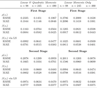
We begin by first considering the case whenxiis arelevantvariable, i.e.,β(zi)6= 0. In particular, the coefficient functions are specified as follows: β(zi) = 1−z2i andρ(zi) = 0.75×sin(πzi). Here, we use a local linear fitting. Table 1 reports the corresponding results for both the first- and second-stage nonparametric GMM estimators fitted using two sets of orthogonality conditions: (i) linear and quadratic moments (left panel) and (ii) linear moments only (right panel).

For each of the two stages, we also report the results for the local linear least squares estimator ofβ(zi) from the equation constructed by moving the endogenous spatial lag termρ(zi)P_j6=iwijyj to the left-hand side of model (2.1) and replacing unknown ρ(zi) with its estimatorρ∗(zi), where the latter equals ρ_b(zi) in the first stage and ρe(zi) in the second stage. It is attractive to explore such a model for likely efficiency gains in finite samples. More concretely, we apply the conventional local linear least squares approach to [In−ρ∗(Z)W]y= mtx{X,β(Z)}+u to obtain, in the local neighborhood ofz:

y∗ _{≈ X}(z)vec_{B(z)_}+u∗, (6.2)

where y∗ _≡ [In−ρ∗(Z)W]y; X(z) = Z1(z)⊗x1 . . . Zn(z)⊗xn′ is an n×[p(q + 1)] data matrix; and B(z) _≡hβ(z) _∇β₁(z) . . . _∇β_p(z)′i. It is easy to show that the resulting non-parametric least squares estimator is given by

vecnB˘(z)o=h_X(z)′KH(z)X(z)

i−1

X(z)′KH(z)y∗. (6.3)

The results in Table 1 indicate that, in all instances, the estimation of both ρ(_·) and β(_·) co-efficients becomes more stable as the sample size increases. Both the RMSE and MAE decline significantly asnincreases. Regardless of the instrument set, as expected, the second-stage estima-tor delivers a sizable improvement over its first-stage counterpart, with a greater impact exhibited for the estimation of ρ(_·). We also observe that adding quadratic orthogonality conditions leads to an increase in accuracy of the first-stage estimator only. Similarly, the reestimation ofβ(_·) via least squares also yields better results in the first stage only.

7

Throughout, to ensure the non-singularity of In−ρ(z)W, we impose (3.11) via either box constraints on ρ(z)

Table 1. Simulation Results for the Estimators whenxi is Relevant

Linear & Quadratic Moments Linear Moments Only

n= 98 n= 245 n= 490 n= 98 n= 245 n= 490

First Stage First Stage

ρ(zi)

RMSE 0.2335 0.1451 0.1067 0.2786 0.2009 0.1638

MAE 0.1844 0.1146 0.0846 0.2096 0.1418 0.1081

β(zi)

RMSE 0.1163 0.0764 0.0564 0.1205 0.0821 0.0598

MAE 0.0884 0.0582 0.0425 0.0917 0.0612 0.0443

β(zi) via LS

RMSE 0.0992 0.0641 0.0477 0.1025 0.0681 0.0509

MAE 0.0791 0.0515 0.0383 0.0811 0.0538 0.0401

Second Stage Second Stage

ρ(zi)

RMSE 0.2078 0.1299 0.0959 0.2011 0.1203 0.0878

MAE 0.1665 0.1034 0.0761 0.1586 0.0960 0.0699

β(zi)

RMSE 0.1010 0.0660 0.0483 0.0994 0.0643 0.0474

MAE 0.0802 0.0528 0.0388 0.0798 0.0516 0.0381

β(zi) via LS

RMSE 0.0974 0.0634 0.0470 0.0975 0.0632 0.0468

MAE 0.0777 0.0508 0.0377 0.0774 0.0507 0.0375

Notes: The reported are the averages of respective statistics over 500 simulations. LS stands for least squares.

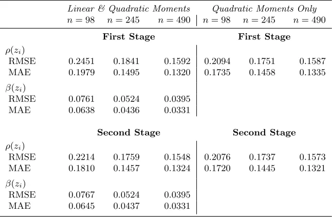
Next, we turn to the case when xi is irrelevant in explaining yi, i.e.,β(zi) = 0. The coefficient functions are specified as follows: β(zi) = 0 for allzi andρ(zi) = 0.75×sin(πzi). In this instance, we estimate our first- and second-stage nonparametric GMM estimators via a local constant approach8 using the following two sets of orthogonality conditions: (i) linear and quadratic moments (left panel) and (ii) quadratic moments only (right panel). The first set of instruments is meant to simulate the case when the researcher is not aware thatβ(zi) = 0, whereas the second set assumes the researcher knows that the model is a pure spatial autoregressive model with no covariates (and hence, only ρ(_·) is estimated).

Table 2 presents the results. Consistent with our theory, all estimators improve with an increase in the sample size. The second-stage estimator offers some gains in the estimation of the ρ(_·) coefficient function primarily only when the model incorrectly presumes that β(z) ₆= 0; no gains are exhibited for β(_·) in this case (left panel of Table 2). In line with one’s intuition, the results indicate that the estimator of a correctly specified pure spatial autoregressive model (right panel of Table 2) outperforms that of a “misspecified” model which includes an invalid instrument Wx in its instrument set.

Overall, simulation experiments lend support to asymptotic results for our proposed estimators.

8

Table 2. Simulation Results for the Estimators when xi is Irrelevant

Linear & Quadratic Moments Quadratic Moments Only

n= 98 n= 245 n= 490 n= 98 n= 245 n= 490

First Stage First Stage

ρ(zi)

RMSE 0.2451 0.1841 0.1592 0.2094 0.1751 0.1587

MAE 0.1979 0.1495 0.1320 0.1735 0.1458 0.1335

β(zi)

RMSE 0.0761 0.0524 0.0395

MAE 0.0638 0.0436 0.0331

Second Stage Second Stage

ρ(zi)

RMSE 0.2214 0.1759 0.1548 0.2076 0.1737 0.1573

MAE 0.1810 0.1457 0.1324 0.1720 0.1445 0.1321

β(zi)

RMSE 0.0767 0.0524 0.0395

MAE 0.0645 0.0437 0.0331

Note: The reported are the averages of respective statistics over 500 simulations.

6.2 Specification Tests

We next examine the small sample performance of our proposed specification tests. As earlier, we consider sample sizes n = _{98, 245, 490_}. For each n, we simulate the model 500 times. Test statistics are bootstrapped 299 times each to obtain the 1%, 5%, 10% and 20% upper percentile (critical) values of their null distributions.

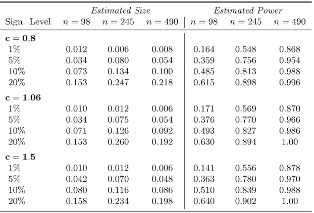
We first study our residual-based statistic Jn. To assess its size and power, we consider the following two experimental designs for the data-generating process given in (6.1):

(i) Linear model: β(zi) = 0.75 and ρ(zi) = 0.5 for all zi.

(ii) Nonlinear model: β(zi) = 1−zi2 and ρ(zi) = 0.75×sin(πzi).

The residuals under the null hypothesis necessary for the construction of Jn are estimated via Lee’s (2007) GMM estimator using the same linear and quadratic instruments as the ones we use in the first-stage estimation in Section 6.1 above. To assess the sensitive of the results to the choice of bandwidth for zi, we try different values of the scale parameter in the Silverman’s (1986) rule-of-thumb bandwidth: c = _{0.80, 1.06, 1.50_}. Table 3 reports the estimated size [design (i)] and power [design (ii)] of our test computed as rejection frequencies over 500 simulations. We find that out test statisticJn exhibits a relatively good size across all considered sample sizes and bandwidth values. From the right panel of Table 3, we also see that the power of the test increases with the sample size as anticipated.

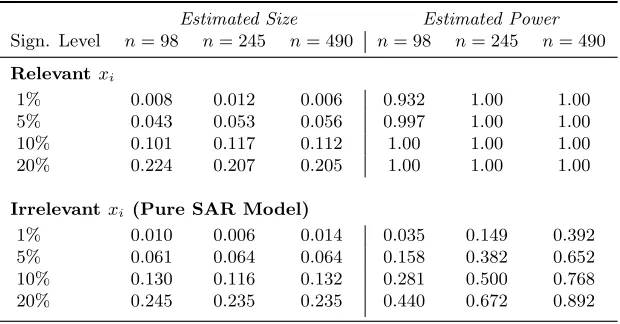
Given that the applicability of the Jn statistic does not extend to the case of pure spatial autoregressive models, we next analyze the performance of our second test statisticDn. To examine its size and power, we consider the following four experimental designs for the data-generating process given in (6.1):

(i) Linear model:

Table 3. Simulation Results for theJn Statistic whenxi is Relevant

Estimated Size Estimated Power

Sign. Level n= 98 n= 245 n= 490 n= 98 n= 245 n= 490

c=0.8

1% 0.012 0.006 0.008 0.164 0.548 0.868

5% 0.034 0.080 0.054 0.359 0.756 0.954

10% 0.073 0.134 0.100 0.485 0.813 0.988

20% 0.153 0.247 0.218 0.615 0.898 0.996

c=1.06

1% 0.010 0.012 0.006 0.171 0.569 0.870

5% 0.034 0.075 0.054 0.376 0.770 0.966

10% 0.071 0.126 0.092 0.493 0.827 0.986

20% 0.153 0.260 0.192 0.630 0.894 1.00

c=1.5

1% 0.010 0.012 0.006 0.141 0.556 0.878

5% 0.042 0.070 0.048 0.363 0.780 0.970

10% 0.080 0.116 0.086 0.510 0.839 0.988

20% 0.158 0.234 0.198 0.640 0.902 1.00

Note: The reported are the rejection frequencies over 500 simulations.

−Irrelevantxi: β(zi) = 0 for allzi and ρ(zi) = 0.5 for allzi. (ii) Nonlinear model:

−Relevant xi: β(zi) = 1−zi2 and ρ(zi) = 0.75×sin(πzi);

−Irrelevantxi: β(zi) = 0 for allzi and ρ(zi) = 0.75×sin(πzi).

We use Silverman’s (1986) rule-of-thumb bandwidth with c = 1.06 throughout. For the case of a relevant xi, both the model under H0 and the model under H1 are estimated using linear and quadratic moments. However, in the case of a pure spatial autoregressive model, we make use of quadratic moments only thus assuming that the irrelevancy ofxi is ana priori knowledge. The results reported in Table 4 show that the Dn test has quite accurate size across alln regard-less whether xi is relevant or not. It exhibits superb power when xi is relevant in predicting yi. The power is also decent and rises with the sample size when the true model is a pure spatial autoregression.

7

Conclusion

Most empirical work that deals with spatial data employs standard linear spatial models. These models are however prone to misspecification due to a rather strong assumption of linearity of the spatial relationship. The literature has long ago recognized that econometric relations in space result more often than not in highly nonlinear specifications.

Table 4. Simulation Results for theDn Statistic

Estimated Size Estimated Power

Sign. Level n= 98 n= 245 n= 490 n= 98 n= 245 n= 490

Relevantxi

1% 0.008 0.012 0.006 0.932 1.00 1.00

5% 0.043 0.053 0.056 0.997 1.00 1.00

10% 0.101 0.117 0.112 1.00 1.00 1.00

20% 0.224 0.207 0.205 1.00 1.00 1.00

Irrelevantxi (Pure SAR Model)

1% 0.010 0.006 0.014 0.035 0.149 0.392

5% 0.061 0.064 0.064 0.158 0.382 0.652

10% 0.130 0.116 0.132 0.281 0.500 0.768

20% 0.245 0.235 0.235 0.440 0.672 0.892

Notes: The reported are the rejection frequencies over 500 simulations. SAR stands for spatially autoregressive.

may be highly desirable from a practitioner’s point of view since it allows the identification of a neighborhood-specific spatial dependence measure conditional on the vector of contextual variables. We propose several (locally) nonparametric GMM estimators for our model. The developed two-stage estimators incorporate both the linear and quadratic orthogonality conditions and are capable of accommodating a variety of data generating processes, including the instance of a pure spatially autoregressive semiparametric model with no relevant regressors as well as multiple partially linear specifications. All proposed estimators are shown to be consistent and asymptotically normal. We also contribute to the literature by putting forward two test statistics to test for parameter constancy in our model. Both tests are consistent.

Appendix

To simplify notation, we define the following: πi ≡ KH(zi, z) =K(H−1(zi−z)); Asn = An+A′n for anyn_×n matrixAn;▽2g(z) =∂2g(z)/∂z∂z′ is the second-order derivative of a differentiable functiong:Rq _→R_{;isand0sis an s×1 vector of ones and zeros, respectively;is×tand0s×t is an}

s_×tmatrix of ones and zeros, respectively;P_{i6=j ≡}Pn_i=1Pn_j6=iandP_{i=j6 6=i}′ ≡Pn_i=1Pn_j6=iPn_j6=i6=i′.

Also, Xn =Oe(an) means that Xn= Op(an) but not Xn =op(an), and An ≈Bn indicates that Bn is the leading term of An.

A

Brief Mathematical Proofs of Theorems 1–4

Proof of Theorem 1. Defineθn=ξn γb(z)−γ(z) [▽bγ(z)− ▽γ(z)]H , a (p+ 1)×(q+ 1) matrix, y∗_i = yi−m′iγ(z)−m′i▽γ(z) (zi−z) and ui(θ) = yi∗−ξn−1m′iθZi(z), where {ξn} is a sequence of positive constants such that 0< M1<kθnk< M2<∞for alln. Then, we can rewrite (3.5) as

gn(θ) =

    

u(θ)′Pn,1KH(z)u(θ) ..

.

u(θ)′Pn,mKH(z)u(θ) Q(z)′KH(z)u(θ)

   

whereu(θ) is ann_×1 vector with a typical element being equal toui(θ). Then, we have

∂gn(θ) ∂vec (θ)′ =−ξ

−1 n

    

u(θ)′[Pn,1KH(z)]sM(z) ..

.

u(θ)′[P_n,lKH(z)]sM(z) Q(z)′KH(z)M(z)

    .

Minimizing the GMM objective function referenced in (3.6) is equivalent to minimizing Λn(θ) = gn(θ)′gn(θ) overθ ∈S, where the latter is a compact subset ofRp+1×Rq+1. Sinceθn minimizes Λn(θ) =gn(θ)′gn(θ), we have that

0_(p+1)(q+1)= ∂gn(θn)

′

∂vec (θ) gn(θn) =

∂gn(θn)′ ∂vec (θ)



gn(0) + ∂gn

e

θn

∂vec (θ)′ vec (θn)

 ,

whereθen lies betweenθn and 0(p+1)(q+1). From above, we obtain

vec (θn) =−



∂gn(θn)′ ∂vec (θ)

∂gn

e

θn

∂vec (θ)′

 

−1

∂gn(θn)′

∂vec (θ) gn(0) .

Denoting ΞH(z) ≡ KH(z)Q(z)Q(z)′KH(z), we decompose the two components of vec (θn) above as follows

An(z) ≡ −

∂gn(θn)′ ∂vec (θ) gn(0)

= 1

2ξn m

X

l=1

M(z)′[Pn,lKH(z)]su(θn)y∗′[Pn,lKH(z)]sy∗+ 1 ξn

M(z)′ΞH(z)y∗

and

Bn(z) ≡

∂gn(θn)′ ∂vec (θ)

∂gneθn

∂vec (θ)′

= 1

ξ2 n

m

X

l=1

h

u(θn)′[Pn,lKH(z)]sM(z)

i′

uθen

′

[Pn,lKH(z)]sM(z) + 1 ξ2 n

M(z)′ΞH(z)M(z).

For each i, we define a (p+ 1)_×1 vector Π(z∗_i) whose lth element equals Πl(z∗i) = (zi − z)′ _▽2 γl(z∗i)(zi −z), and z∗i lies between zi and z for l = 1, . . . , p+ 1. Then, we have yi∗ = ui +m′iΠ(z∗i)/2. Further, we define an n×1 vector C(z), whose ith term equals m′iΠ(z∗i)/2, along with Γ1,l = u′[Pn,lKH(z)]sC(z), Γ2,l = C(z)′[Pn,lKH(z)]sC(z), Γ3,l =u′[Pn,lKH(z)]su, Ψ1,l =u′[Pn,lKH(z)]sM(z), Ψ2,l =C(z)′[Pn,lKH(z)]sM(z) and Ψ3,l =M(z)′[Pn,lKH(z)]sM(z) forl= 1, . . . , m. Then, we have An(z) =An1(z) +An2(z)−An3(z) with

An1(z) = 1 2ξn

m

X

l=1

Γ2,l(Ψ1,l+ Ψ2,l)′+ (2Γ1,l+ Γ3,l) Ψ′1,l

+ 1 ξn

M(z)′ΞH(z)C(z)

An2(z) = 1 2ξn

m

X

l=1

(2Γ1,l+ Γ3,l) Ψ′2,l+ 1 ξn