Conditioning a Markov chain upon the behaviour of an additive functional

(1)

warwick.ac.uk/lib-publications

A Thesis Submitted for the Degree of PhD at the University of Warwick

Permanent WRAP URL:

http://wrap.warwick.ac.uk/103716

Copyright and reuse:

This thesis is made available online and is protected by original copyright. Please scroll down to view the document itself.

Please refer to the repository record for this item for information to help you to cite it. Our policy information is available from the repository home page.

(2)

Conditioning a Markov chain upon the

behaviour of an additive functional

Zorana N ajdanovic

A thesis submitted for the degree of Doctor of Philosophy

Department of Statistics

University of Warwick

Coventry

CV47AL

(3)

<

Ho}

3.2 Conditioning the process (Xt,<Pt)t~O on the event {Ho

>

T}

4 The negative drift case

4.1 Conditioning the process (Xt,<ptk~o on the event {Hy

<

Ho}

4.2 Conditioning the process (Xt, <ptk::o on the event {Hy

<

+oo} 4.3 Conditioning the process (Xt, <Pt)t~O on the event {Ho

>

T}

4.4 Conditioning the process (<ptk::o to oscillate.

5 Conclusions

A The Perron-Frobenius theorems

B The proofs of auxiliary lemmas

ii

107 110

112

113 125

133

135 141 151 170

174

179

(5)

List of Figures

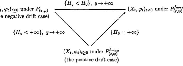
1.1 A typical path of the process (Xt, cptk:o starting at (e, cp) E Ed" • . 14 1.2 The Perron-Frobenius eigenvalue o:(f3) of the matrix (Q - f3V) .. 55 5.1 The negative drift case of conditioning the process (Xt , CPt)(~O on the

events {Hy

<

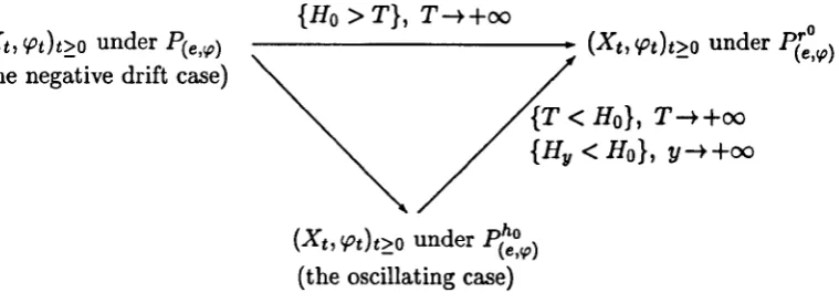
Ho}, y ~ O. . . .. 177 5.2 The negative drift case of conditioning the process (X_{t, cpdt;::o on the}

events {Ho

>

T}, T ~ O. . . .. 178

(6)

Acknowledgements

I wish to thank my family and friends from Yugoslavia for their full support over the past three years.

I am also grateful to the members of the Department of Statistics for creating such a warm and working atmosphere and to all my Warwick friends, especially to Bice, Elke,

Anna and colleagues in Room 66, for their friendship,understanding and support. Above all, I am endlessly grateful to my supervisors Dr Saul Jacka and Dr Jon Warren for their enthusiasm, invaluable guidance, encouragement and enormous patience which led me to the completion of this thesis.

This research was supported by the Overseas Research Student award and by the

Special Student Research award.

(7)

Declaration

I hereby declare that this thesis is my own work completed under the guidance of my

supervisors Saul D Jacka and Jon Warren and has not been submitted for a degree at another university.

(8)

Abstract

We consider a finite statespace continuous-time irreducible Markov chain (Xtk::o to-gether with some fluctuating additive functional (ct't)t;::o. The objective is to condition the Markov process (Xt, IPt)t;::o on the event that the process (IPth;::o stays non-negative. There are three possible types of behaviour of the process (IPt)t;::o: it can drift to

+00,

oscillate, or drift to

-00,

and in each of these cases we condition the process (Xt, IPt)t;::o

on the event that the process (ct'th;::o stays non-negative.

In the positive drift case, the event that the process (IPt)t;::o stays non-negative is of positive probability and the process (XI! ct'th;::o can be conditioned on it in the standard way. In the oscillating and the negative drift cases, the event that the process (IPt)t;::o

stays non-negative is of zero probability and we cannot condition the process (Xt, IPdt;::o

on it in the standard way. Instead, we look at the limits of laws of the process _{(Xt, IPt)t;::o} conditioned on the event that the process (lPdt;::o hits large levels before it crosses zero,

and of laws of the process (Xt, ct't)t;::o conditioned on the event that the process (IPt)t;::o

stays non-negative for a large time. In the oscillating case both limits exists and are equal to the same probability law. In the negative drift case, under certain conditions, both limits exist but give distinct probability laws.

In addition, in the negative drift case, conditioning the process (Xt, IPt)t;::o on the event that the process (<pt)t;::o drifts to

+00

and then further conditioning on the event that the process (lPdt;::o stays non-negative yields the same result as the limit of con-ditioning the process _{(Xt, IPt)t;::o}on the event that the process (ct'th;::o hits large levels before it crosses zero. Similarly, conditioning the process (X_{t ,}IPth>o on the event that the process {lPt}t;::o oscillates and then further conditioning on the event that the process

{lPdt;::o stays non-negative yields the same result as the limit of conditioning the process

(Xt, <Pt)t;::o on the event that the process (<pt)t~O stays non-negative for a large time.

(9)

Frequently Used Notation

Q

E

J.'

V E+ E-

_,

r,G

n-,n+

c+,G-aj, j = 1, ... ,n

{3k, k = 1, ... ,m

The Q-matrix of the process (Xt)t2:0 (page 14).

The statespace of the process (Xtk:o (page 14).

The invariant measure of the process (Xe)t2:0 (page 14). The diagonal matrix diag(v(e)) (page 14).

The sets v-1(O,+oo} and v-1(-oo,O} (page 14). The halfspaces (E x (y,+oo))

U

(E+ x {y}} and

(E x (-oo,y))

U

(E- x {y}} (page 15).

The first crossing time of the level y by the process ('Pt}t2:0 (page 15).

The matrices given by the Wiener-Hopf factorization of the matrix V-1Q (page 18).

The components of the matrix

r

(page 18). The components of the matrix G (page 18).

The matrices given by the Wiener-Hopf factorization of the matrix V-1(Q - al}, a> 0 (page 16).

The components of the matrix

r

0, a> 0 (page 16).

The components of the matrix Go, a

>

0 (page 16). The eigenvalues of the matrix V-1Q with non-positive real parts (page 26).

The eigenvalues of the matrix V-1Q with non-negative real parts (page 26).

(10)

O'max

f3min

Ii,

j

=

1, ... ,n

9k, k

=

1, ... ,~

fmax

9min

The eigenvalue of the matrix V-1Q with maximal non-positive real part (page 26).

The eigenvalue of the matrix V-1Q with minimal non-negative real part (page 26).

Vectors associated with the eigenvalues of the matrix V-1Q with non-positive real parts (page 26).

Vectors associated with the eigenvalues of the matrix V-1Q with non-negative real parts (page 27).

The eigenvector of the matrix V-1Q associated with the eigenvalue O'max (page 28).

The eigenvector of the matrix V-1Q associated with the eigenvalue f3min (page 28).

Matrices defined on pages 29 and 30.

(11)

Introduction

The problem of conditioning a stochastic process to stay forever in a certain region has been extensively studied in the literature. Many authors have addressed the essentially same problem by conditioning a process with a possibly finite lifetime to live forever.

An interesting case is when the event that the process remains in some region is of zero probability, or in terms of the lifetime of the process, when the process has a finite lifetime with probability one. In that case we cannot condition the process to stay in the region forever in the standard way. Instead, we can look at the limit of conditioning the process to stay in the region for a large time or at the limit of conditioning the process to stay away from the boundary of the region.

There are many well-known examples of such conditionings. For instance, Knight [24] in 1969 showed that the standard Brownian motion conditioned not to cross zero for a large time converges weakly to a three-dimensional Bessel process; Iglehart [16]

in 1974 considered a general random walk conditioned to stay non-negative for a large time and showed that it converges weakly; Williams [34] in 1974 showed that Brownian motion conditioned to hit level y before hitting zero converges weakly as y ~ +00

to a three-dimensional Bessel process, which is the same limit as of Brownian motion conditioned not to cross zero for a large time. Williams also showed that Brownian motion with a negative drift conditioned to hit level y converges weakly as y ~ 00 to

Brownian motion with a positive drift; Pinsky [27] in 1985 showed that under certain conditions, a homogeneous diffusion on

r

conditioned to remain in an open connected

bounded region for a large time converges weakly to a homogeneous diffusion; Jacka and

Roberts [36] in 1988 proved weak convergence of an Ito diffusion conditioned to remain in an interval (a, b) until a large time.

(12)

INTRODUCTION 2

counterexamples in which a process conditioned to stay in a region for a large time does not converge at all or it does converge but to a dishonest limit. Jacka and Warren [21] in 2002 gave two examples of such processes.

Dertoin and Doney [4] in 1994 considered a real-valued random walk {Sn, n ~ O} and discussed these two ways of conditioning it to stay non-negative. Namely, they looked at the limit when n -+ 00 of conditioning {Sn, n ~ O} on the event

A~l)

= { {Sn,

n

~

O} hits

[n,

+00) before it hits (-00,0) },

that is the event that {Sn, n ~ O} hits at least level n before crossing zero, and at the

limit when n -+ 00 of conditioning {Sn, n ~ O} on the event

A~2)

= { Sk

~

0 for all 0

:S

k

:S

n},

that is the event that {Sn, n ~

O}

stays non-negative until time n. They showed that - when the random walk oscillates, these two ways of conditioning yield the same

honest limit;

- when the random walk drifts to -00, then under a certain condition the two ways of conditioning yield distinct honest limits, but if the upper tail of the step distribution is slowly varying, then the two ways of conditioning yield the same dishonest limit;

- under a certain condition, the random walk {Sn,n ~ O} with a negative drift conditioned On the event {{Sn, n ~ O} hits [n, +oo)} converges weakly as n -+ +00 to a random walk with a positive drift and then further conditioning the resulting random walk with a positive drift on the event that it stays non-negative yields the

same result as the limit as n -+ +00 of conditioning the random walk {Sn, n ~

O}

on the event A~l);

(13)

INTRODUCTION 3

to an oscillating random walk, and further conditioning this oscillating random walk on the event that it stays non-negative yields the same result as the limit as n ~ +00 of conditioning the random walk {Sn, n ~ o} on the event A~2).

These results by Bertoin and Doney for a random walk were the motivation and the starting point for our work. Instead of considering a random walk {Sn, n ~ o} we study a finite statespace continuous time Markov chain and an associated fluctuating additive functional, and want to condition the Markov chain on the event that the fluctuating functional stays non-negative.

More precisely, let X = (Xt)t~O be an irreducible Markov chain with statespace E and let v be a map v: E --+ 1R\{O}. Suppose that both E+ = v-1(O,00) and E- = v-1(-00,O) are non-empty. Define the process (cpt)t~O by

CPt

=

cP

+

fot v(X,,)ds,

where cP E IR is some non-random initial value for CPO.

The objective is to condition the process (Xt, CPt)t~O starting at (e, cp) E Ex (0, +00) or (e, cp) E E+ x {O}, on the event that the process (cpth~o stays non-negative. We distinguish between three possible cases: when the process (cpt)t~O drifts to +00, when it oscillates and when it drifts to -00 and perform conditioning in each of the cases separately.

The behaviour of the process (cpt)t~O is completely determined by the matrix Q and the function v and is related to the processes obtained from the process (Xt)t~O via time substitutions based on the process (cpt)t~o. Namely, for stopping times T+ and T- given

by

T:

= inf

{t

>

0 : CPt

>

Y}

Ty

= inf{t

>

0 : CPt

<

-y}.

(14)

INTRODUCTION 4

the Wiener-Hopf factorization for Markov chains. The Wiener-Hopf factorization has various meanings for various processes. For instance, the Wiener-Hopf factorization for Levy processes (see Rogers [29]) gives the relation between a Levy process and its running maximum and minimum; the Wiener-Hopf factorization for diffusions (see Rogers [29]) involves processes obtained from a diffusion by time changing; the

Wiener-Hopf factorization for random walks has many formulations (see Alili and Doney [1]) but it always involves the ladder times and the ladder heights processes associated with

a random walk.

The Wiener-Hopf factorization for matrices and its probabilistic interpretation in the theory of Markov chains (see Williams [36], Barlow, Rogers, Williams [3], London, McKean, Rogers, Williams [26]) is a very powerful tool for obtaining and proving results for Markov chains. As will be seen, the Wiener-Hopf factorization of the matrix V-1Q, where the matrix V is the diagonal matrix diag(v(e» and the matrix Q is the Q-matrix of the process (Xth~o, plays a prominent role in our work since most of the results

are based on it and its consequences. Because of that, a whole section (Section 1.4) is dedicated to the study of the Wiener-Hopf factorization of the matrix V-1Q and its implications. Other major techniques and tools used are the theory of martingales,

the theory of Laplace transforms, the Tauberian theorems and the Perron-Frobenius theorems.

The thesis is organized into six chapters. Chapter 1 is preliminary and is intended

to introduce the notation and prepare for the results in the following chapters. The first two sections in Chapter 1 contain matrix definitions and some auxiliary matrix lemmas.

The process (Xt, CPt)t~O which is the basic object in our work is introduced in Section 1.3.

Section 1.4 is, as previously mentioned, concerned with the Wiener-Hopf factorization

(15)

INTRODUCTION 5

1.6 the generator of the process (Xt, 'Ptk~o, and in Section 1.7 the behaviour of the process ('Pt)t;::o. Results in Sections 1.8 and 1.9, about the eigenvalues of the matrix V-1(Q - 01), 0 ~ 0, and h-transforms of the process (Xt, 'Pt)t;::o, are used in Chapters 3 and 4. In Section 1.10 we start with conditioning the process (Xt, <Pt)t;::o on the event that the process ('Pth;::o stays non-negative. The first and the easiest case, when the process {'Pt)t;::o drifts to

+00,

is discussed in Section 1.10. In that case, the event that the process ('Pt)t;::o stays non-negative is of positive probability and the process (Xt, 'Pth;::o

can be conditioned on it in the standard way.

Chapter 2 deals with the Green's functions of the process (Xt, 'Pt)t;::o and of the process {Xt, 'Pt)t;::o killed when the process {'Pt)t;::o crosses zero. We present several ways for calculating them and show the variety of ideas and techniques that are used.

In Chapter 3 we look at conditioning the process (Xt, 'Pth;::o on the event that the process ('Pt)t;::o stays non-negative when the process ('Pt)t;::o oscillates. In that case, the event that the process ('Pth;::o stays non-negative is of zero probability and

conditioning the process {Xt, 'Pt)t;::o on it is not possible in any elementary way. Instead, we approximate the event that the process ('Pt)t;::o stays non-negative by some events of positive probabilities, and look at the limit of conditioning (Xt, 'Pt)t>o on those events. We discuss conditioning the process (Xt, 'Pt)t;::o on two approximations of the event that the process {'Pth;::o stays non-negative: in Section 3.1 on the approximation by the events that the process {'Pt)t;::o hits large levels before it crosses zero, and in Section 3.2

on the approximation by the events that the process ('Pdt;::o stays non-negative for a large time.

In Chapter 4 we finally look at the most interesting case of conditioning the process

{Xt, 'Pt)t;::o on the event that the process ('Ptk~o stays non-negative, that is the case when

(16)

INTRODUCTION 6

process (Xt, If'tk~o on it, we look (in Section 4.1) at the limit of conditioning the process

(Xt, If'tk~o on the event that the process (If'tk~o hits large levels before it crosses zero, and (in Section 4.3) at the limit of conditioning the process (Xt,

If'tk::o

on the event that the process (If'tk::o stays non-negative for a large time. In addition, in Sections 4.2 and 4.4, we make two more transformations of the process (Xt, If'tk~o in order to change the behaviour of the process (If'th;::o, and we look at relations between the processes obtained in these two transformations and the original process (Xt, If't}t;::o. Our objective is to obtain the results analogous to those obtained by as Bertoin and Doney (1994) for a random walk (which have been listed above).

(17)

Chapter

1 Preliminaries

In this chapter we introduce the notation and review some results and prove some other results that will be used in following chapters.

1.1 Conventions and some matrix lemmas

By positive we mean "

>

0 ". By negative we mean "

<

0 ". By non-positive we mean " ~ 0 ". By non-negative we mean " ~ 0 " .

We denote the d x d identity matrix by I where the dimension d varies from line to line and is meant to be clear from context.

All equalities and inequalities between vectors or matrices are meant componentwise. Let A be a square matrix and a its eigenvalue. We say that a non-zero vector 9 is associated with the eigenvalue a if there exists n E N such that

if 9 is a column vector, or

g(A - aJ)n

=

0

if 9 is a row vector. By Jordan normal form theory, the number of independent column

(18)

CHAPTER 1. PRELIMINARIES 8

vectors (or row vectors) associated with the same eigenvalue is equal to the algebraic multiplicity of the eigenvalue.

Lemma 1.1.1 Let a and

/3,

a -=F

/3,

be eigenvalues of a square matrix M.

(i) Let 9 be a row eigenvector of the matrix M associated with the eigenvalue a, and let

f be a column vector associated with the eigenvalue

/3.

Then gf = 0;

If 9 is a column eigenvector of the matrix M associated with the eigenvalue a, and f is

a row vector associated with the eigenvalue

/3,

then fg = OJ

(ii) Let a be a simple eigenvalue of M. If 9 and f are left and right eigenvectors,

respectively, of M associated with the eigenvalue a, then gf

=f

O.

Proof: (i) Let kEN such that (M - /3I)k f = O. Then, because g(M - aI) = 0,

o

= g{M - /3I)k

f

= g((M - aI)

+

{a - /3)1)k /

k

= 9

L

(~)

(M - aI)i (a - /3)k-i /

j=O J

= (a - /3)k

g/,

and because a -=F

/3,

9

=f

0 and /

=f

0, gf = O. the statement for a column vector 9 and a row vector / can be proved in the same way.

(ii) By Jordan normal form theory, there exists a basis S in the space of all vectors on

IR" which consists only of vectors associated with the eigenvalues of the matrix lvI. If

a is a simple eigenvalue, then there is only one vector in the basis S associated with a and that is its associated right eigenvector /. By (i), the vector g, a left eigenvector of M associated with a, is orthogonal to all vectors in the basis S which are not equal to /. If also

g/

= 0 , then 9 is orthogonal to all vectors in the basis S which implies that

9 = O. But 9 -=F 0 since it is a left eigenvector of M. Therefore,

g/

-=F O.

o

(19)

A Q-matrix is an essentially non-negative matrix with non-positive row sums. If all row sums are equal to zero then the Q-matrix is called conservative.

A square non-negative matrix is called substochastic if all row sums are less than or equal to 1, strictly substochastic if it is substochastic and at least one row sum is strictly less than 1, and stochastic if all row sums are equal to 1.

A square non-negative matrix is called primitive if there exists kEN such that Tk is a positive matrix.

Let i be arbitrary index from them index set {I, 2, ... n} of the non-negative matrix T. Suppose that there exists mEN such that TtJ is positive. Then, the period d(i) of the index i is the greatest common divisor of those k for which Ti~i is positive.

A square non-negative matrix T is called irreducible if for every pair i, j of its index set, there exists kEN such that Ti~i is positive. An irreducible matrix is said to be cyclic with period d if the period of anyone (and so of each one) of its indices satisfies

d> 1, and is said to be acyclic if d = 1.

Lemma 1.1.2 A square non-negative matrix is irreducible and acyclic if and only if it is primitive.

Proof: See Theorem 1.4. in Seneta [31].

o

An essentially non-negative matrix B is associated with a non-negative matrix T through the relation

T=B+cI,

for some positive real constant c. An essentially non-negative matrix B is called irre-ducible if its associated non-negative matrix T is irreducible.

The Perron-Frobenius theorems for primitive matrices and for irreducible essentially

(20)

One of the implications of the Perron-Frobenius theorems for primitive matrices and for irreducible essentially non-negative matrices is that there exist simple eigenvalues of such matrices with which can be associated positive right and left eigenvectors. This fact together with Lemma 1.1.1 proves

Lemma 1.1.3 The Perron-Frobenius left and right eigenvectors of a primitive matrix are the only positive vectors associated with the eigenvalues of the matrix.

The same statement is true for an irreducible essentially non-negative matrix.

Proof: Let T be a primitive matrix. By the Perron-Frobenius theorems for primitive matrices there exists a simple eigenvalue a of T such that left g/eft and right gright

eigenvectors associated with a are positive. Let f left and right be a row and a column vector, respectively, associated with an eigenvalue

f3

ofT where

f3

t=

a. Then, by Lemma 1.1.1 (i), g/eft right

=

0 and f'eftgright

=

0, and because gleft and gright are positive, it follows that the vectors f 'eft and right cannot be positive. Hence, the only positive vectors associated with the eigenvalues of T are its Perron-Frobenius eigenvectors.

The only property of the primitive matrix T that is used in the proof is that it has a simple eigenvalue with which can be associated positive right and left eigenvectors. Since an irreducible essentially non-negative matrix has the same property, it follows that the statement in the lemma which was proved for primitive matrices is also valid for irreducible essentially non-negative matrices.

o

We give three more lemmas, the first of which is proved in Seneta [31].

Lemma 1.1.4 An essentially non-negative matrix Q is irreducible iff etQ is positive for all t

>

O.

(21)

CHAPTER 1. PRELIMINARIES

Lemma 1.1.5 Let Q be an irreducible Q-matrix. Then

etQl = 1 for some t

>

0 iff etQl = 1 for all t ~

o.

In addition,

Q

is conservative iff etQ _{is stochastic for all}_t_~₀

Q is not conservative iff etQ 1

<

1 for all t

>

O.

11

Proof: For the first part of the lemma, it is enough to show that if etQ 1 = 1 for some

t

>

0 then etQ ₁₌_{1 for all}_{t ;:::}_O.

Differentiating etQ lover t we obtain

de;:1

=

e

tQ_Q1.

Since Ql

:5

0 and, by Lemma 1.1.4, etQ is positive for all t

>

0, the last equation implies that de~~l

:5

0 which means that the function t H etQl is decreasing.

Suppose that etoQl

=

1 for some to

>

O. Then, esQl = 1 for all 0

:5

s

<

to. If t

>

to

then there exists kEN such that (k - l)to

<

t

:5

kto. Thus, for such t,

Therefore, etQ 1 = 1 for all t ;:::

o.

For the second part of the lemma, we first notice that

Ql = 0 iff etQl = 1 for all t ~

o.

Hence, all we have to prove is that if Q is not conservative then etQ 1

<

1 for all t

>

o.

Suppose that Q is not conservative. Then, etQ is strictly substochastic for some

t

>

0, which, by the first part of the lemma, implies that etQ is strictly substochastic for all t ;::: O. By Lemma 1.2.1, etQ

>

0 for all t

>

O. Hence, for any t

>

0,

(22)

CHAPTER 1. PRELIMINARIES 12

Lemma 1.1.6 Let Q be an irreducible essentially non-negative matrix, V a diagonal

matrix and f3 E Ilt Then the matrix (Q - f3V) is essentially non-negative matrix and

irreducible.

Proof: The matrices Q and (Q - f3V) are essentially non-negative which implies that there exists sufficiently large real constant c such that the matrices

T= Q+cI and S = Q - f3V +cI

are non-negative and have positive entries on the main diagonal. Since the matrices T and S have positive entries and zero entries in same positions, it is also valid for all their powers Tk and Sk, kEN. Thus the matrix T is primitive if and only if the matrix S is

primitive.

Since the matrix Q is irreducible, the matrix T is also irreducible, and because all

its diagonal entries are positive it is also acyclic. Thus, by Lemma 1.1.2, the matrix

T is primitive. We conclude that the matrix S is primitive which, again by Lemma

1.1.2, implies that the matrix S is irreducible. Therefore, by the definition, the matrix

(Q - f3V) is irreducible. 0

1.2 Irreducible Markov chains

Let (Xt)t~O be a Markov chain on a finite statespace E and let Q be its Q-matrix, that is, for all t

2:

0,

Pe(Xt

=

e')

=

etQ(e,e'), e,e' E E,

where Pe(Xt

=

e') denotes the probability that the process (Xt)t~O starting at the state

e is at the state e' at time t.

(23)

Lemma 1.2.1 Let Q be the Q-matrix of a Markov chain (Xtk:~o on a statespace E.

Then

(Xtk::o is irreducible iff the matrix Q is irreducible.

Proof: Dy the definition, the Markov chain (Xtk~o is irreducible if for every e, e' E E

there exists t

>

0 such that

-the 'if' part: if the matrix

Q

is irreducible, then by Lemma 1.1.4 the matrix etQ is positive for all t

>

0 and therefore the chain (Xtk::o is irreducible.

-the 'only if' part: let e, e' E E and suppose that etoQ(e, e')

>

0 for some to.Let

T=Q+cI

for some constant c such that the matrix T is non-negative. Then

(1.1)

(1.2)

Since e-cto

>

0 and t~

>

0, k ~ 0, there exists kEN such that Tk (e, e')

>

O. Thus, for any e,e' E E, there exists kEN such that Tk(e,e')

>

0, which by definition means that the matrix T is irreducible and therefore, the matrix Q is also irreducible. 0

(24)

Let E, Q and J.L denote a finite statespace, the conservative irreducible Q-matrix and the unique invariant probability measure, respectively, of the Markov chain (Xt)f~O.

Let v be a map v:E ---+ 1R\{O} and let V be the diagonal matrix diag(v(e)). Suppose that both E+=v-1(O,oo) and E-=v-1_{(-oo,O) are non-empty and that}

IE+I

₌_nand

IE-I

= m for some n,m E N.

Define the process (rpt)t~O by

rpt

=

rp

+

fot

v(X,)ds,

where rp E IR is the starting point of the process (rpe)t~o.

By the definition, the process (rpt)t~O is increasing when the process (Xt)t~O is in E+ and decreasing when the process (Xth~o is in E-. A typical path of the process (Xt, rpt)t~O is as shown in the diagram in Figure 1.1.

e

I

rp _I

( rpt)

E

-Figure 1.1: A typical path of the process (Xt,<Pt)t~O starting at (e,rp) E Ed

(the values of the process (rpt)t~O are given on the x-axis and the states of the process

(Xt)t~O are given on the y-axis)

[image:24.534.90.425.403.575.2]

(25)

starting at (e, cp), that is

p(e,<p)( • )

=

P( •

I

Xo

=

e, CPo

=

cp),

and let E(e,<p) denote the expectation operator associated with the probability measure

p(e,<p) •

For y

2::

0 define the stopping times

7':

= inf {t

>

0 : CPt

>

y}

7'; -

inf{t

>

0 : CPt

<

-y}.

For the process (cpth~o starting at zero define the processes y+ = (Y!I+)Y~o and Y- = (Yy-)y~o by

The irreducibility of the process (Xt)t~O implies that the processes Y+ and Y- are

also irreducible Markov chains, which will be proved in the following section. Let

E:

and E

_y,

Y E lR, be the halfspaces

E: = (E

x

(y, +00))

U

(E+ X {y}),

E:;; = {E

x

(-oo,y))

U

(E-

x {y}).

In the sequel we shall always assume that the process (Xt, CPt)t~O starts at (e, cp) E

Ed,

unless otherwise stated.

Let Hy , y E lR, be the first crossing time of the level y by the process (cpt)t~O defined

by

{

inf {t

>

0 : CPt

<

y}

H

y =

inf {t

>

0 : CPt

>

y}

if {Xt, CPt)t~O starts in

E:

if {Xt, CPt)t~O starts in E

y.

If the process (Xt,CPt)t~O starts at (e,cp) E

Et,

then because the process (cpt)t~O is continuous, the only possible way for the process (cpt)t~O to enter the negative half-line

(26)

and {Ho = +oo} are equal. In the sequel we shall use this equality without further comment.

Before we close the section, we introduce vector notation that will be constantly in

:::

i:~h:e:;::t:~l:~r

:::::::::

::u:~l:~:r

";:9:

~e(::

)

~:t:~:i::

:::

I-' as I-'

=

(J.L+ 1-'-).

The constant vector g(e) = 1, e E E, is denoted by 1 and for fixed e E E, Ie denotes the indicator of e.

1.4 Wiener-Hopf factorization for matrices

The main tool in approaching the problems and obtaining results in the presented work

is Wiener-Hopf theory. In this section we introduce the Wiener-Hopf factorizations of the matrices V-I (Q - 01), 0 ~ 0, and discuss some of their implications.

Let 0 be a positive real number. We state two lemmas which were proved in Barlow

et al. [3]:

Lemma 1.4.1 For fixed 0

>

0, there exists a unique pair

(nt,

n~), where

nt

is an

E- x E+ matrix and n~ is an E+ x E- matrix, and there exist Q-matrices Gt and

G~ on E+ x E+ and E- x E-, respectively, such that, if

_ (1

n~)

ra

-n+

_a 1 (

G+

and Ga

= ;

then

r

a is invertible and

(27)

Lemma 1.4.2 Let a

>

0 be fixed. Then

E(e,o)(e-oHoI{XHo

=

e'}) = nt(e, e'), (e,e') E E- x E+,

E(e,o)(e-OHOI{XHo

=

e'})

-

rr~(e, e'), (e,e') E E+ x E-,

E(e,o)(e-oHIII{XH_JI = e'}) = e.yGt (e, e'), (e,e') E E+ x E+, y

>

0,

E(e,o)(e-oH-JlI{XH_

JI = e'}) = e yG;; (e, e'), (e,e') E E- x E-, y

>

O.

Lemma 1.4.1 is said to yield the Wiener-Hopf factorization of the matrix Vl(Q -aI).

The following results were also shown in Barlow et al. [3]: The matrix V-1(Q - aJ)

cannot have strictly imaginary eigenvalues and there exists a basis B(a) in the space of all vectors on E which consists only of vectors associated with the eigenvalues of the matrix V-1(Q - aI), that is if g(a) is a vector in B(a), then

(1.3)

for some eigenvalue ).(a) of V-1(Q - aI) and some kEN. The number of vectors in

the basis 8(a) associated with the same eigenvalue is equal to the algebraic multiplicity of that eigenvalue.

Let N(a) and P(a) be the sets of vectors g(a) E 8(a) associated with eigenvalues with positive and with negative real parts, respectively. Then, if the vector g(a) is in

N(a), it is of the form

(

g+(a) )

g(a) = ntg+(a) , (1.4)

and if the vector g(a) is in P(a), it is of the form

(1.5)

The set N(a) contains exactly IE+I

=

n vectors and the vectors g+(a) for all g(a) E

N(a) form a basis in the space of all vectors on E+, and the set P(a) contains exactly

(28)

of all vectors on E-. The eigenvalues of V-l(Q - aI) with strictly negative real part coincide with the eigenvalues of Gt, and the eigenvalues of V-1(Q - aI) with strictly positive real part coincide with the eigenvalues of

-G-;..

The case a = 0 in Lemmas 1.4.1 and 1.4.2 has also been discussed in Barlow et aZ.

[3] and the following lemma, which yields the Wiener-Hopf factorization of the matrix V-lQ, has been proved.

Lemma 1.4.3 There exists a unique pair (11+,11-), where 11+ is an E- X E+ matrix

and 11- is an E+ X E- matrix, and there exist Q-matrices G+ on E+ X E+ and G- on

E-

x

E- such that

(1.6) where

r=

(:+

~-)

and

G=

C+ _:_).

Moreover, n+ and 11- are substochastic and

p(e,O) (Xll0

=

e'}

=

11+(e, e'}, (e,e') E E- x E+, p(e,O) (X 110

=

e')

-

n-(e,e'), (e,e') E E+ x E-,

p(e,O) (XllJ1

=

e')

-

eyG+ (e, e'), (e,e') E E+ x E+, y ~ 0, p(e,O)(Xll__JI= e')

_-

eyG - (e, e'), (e,e') E E- x E-, Y ~O.

The irreducibility of the chain (Xth~o implies that the matrices n+ and 11-, defined in the previous lemma, are positive. This is proved in the next lemma.

Lemma 1.4.4 (i) The matrices 11- and n+ are positive.

(ii) The matrices (11+n- - I) and (11-11+ - I) are essentially non-negative and irre-ducible.

(29)

We shall prove that the matrix 11- is positive.

Let the process (Xtk~:o start at the state e and leave it at time

t.

Then during time 8 such that 0

<

8

<

Imin{v(:):~EE-}1

the process (IPtk::o cannot reach zero. On the other hand, during the same time 8 the process (Xtk~o can jump into the state e' and after the jump it can stay in e' long enough for the process (IPt)t2:0 to hit zero. Hence,

00 tv(e)

, {{lmin{v(el.eeE-}1 (

p(e,O)(XHo

=

e) ~

10 10

p(e,O) (Xt)t2:0 leaves the state

e in time dt, it is in the state e' at time 8 and after time 8 it stays in e' at least for the time

tv(e)

+

s max{v(e}, e E E+})d d

Iv(e')1 s t

00 tv(e)

- 10

lo'min{V(el,eeE}I (-Q(e, e)) etQ(e,e) esQ(e, e')

tv(e)+. max{v(e),ee E+} Q(e' e')

e Iv(e'li ' ds dt

>

O.

Hence, for all (e,e') E E+ x E-, p(e,O)(XHo

=

e')

=

rr-(e,e')

>

O.

It can be proved in the same way that the matrix 11+ is positive.

(ii) Dy (i), the matrices l1+n- and rr-rr+ are positive. It folows that they are primitive, and, by Lemma 1.1.2, irreducible. Therefore, the matrices (n+n- - J) and (l1-n+ - I)

are essentially non-negative and irreducible.

o

The matrix

r

defined in Lemma 1.4.3 is not necessarily invertible. More precisely,

Lemma 1.4.5 If the matrices rr+ and rr- are both stochastic, then the matrices (1 -l1-n+), (I - 11+11-) and r are not invertible.

If at least one of the matrices rr+ and n- is strictly substochastic, then the matrices

(J - rr-n+), (1 - rr+rr-) and r are invertible and the inverse r- 1 is given by

(

(J - rr-n+)-1 -n-(1 - n+n-)-I) .

r-

1

--11+(1 - 11-11+)-1 (I - n+I1-)-1

(30)

Proof: Suppose that n+ and n- are stochastic matrices. Then (1 - n-n+)l + = 0,

r ( 1 + )

=

(1

n-) ( 1 + )

=

(1 + - n-1-)

=

0,

-1- rr+ 1 -1- rr+1+

-1-which shows that none of the matrices

(i -

rr-rr+), (I - rr+rr-) and

r

is invertible. Suppose now that at least one of the matrices rr+ and rr- is strictly substochastic, that is rr+ 1 + $ 1-or rr-1- $ 1+ with strict inequality in at least one entry. By Lemma

1.4.4 (i), the matrices rr+ and rr- are positive which implies that (rr-rr+ - 1)1+ $ 0 and (rr+rr- - 1)1- $ 0 with strict inequality in at least one entry. In addition, By Lemma 1.4.4 (ii), (rr-rr+ - 1) and (rr+rr- - 1) are irreducible essentially non-negative matrices. Thus, the Perron-Frobenius theorem for irreducible essentially non-negative matrices implies that the Perron-Frobenius eigenvalues of the matrices (n-rr+ - 1) and

(rr+rr- - 1) are negative. Thus, the matrices (rr-rr+ - 1) and (rr+rr- - 1) do not have zero as an eigenvalue and therefore they are invertible. Moreover, by the same theorem, the inverses (1 - rr-rr+)-l and (1 - rr+rr-)-l are positive.

Finally, directly checking shows that the matrix

(

(I - rr-rr+)-l -n+(I - rr-n+)-l

is the inverse of the matrix

r.

-rr-(I - rr+rr-)-l) (1 - rr+rr-)-l

Another immediate consequence of Lemma 1.4.3 is

Lemma 1.4.6 (i) The matrices G+ and G- are irreducible Q-matrices.

(ii) G+ is conservative iff rr+ is stochastic

G- is conservative iff rr- is stochastic.

o

Proof: (i) By Lemma 1.4.3, the matrices G+ and G- are the Q-matrices. In order to prove that they are irreducible, by Lemma 1.1.4 it is enough to prove that the matrices

(31)

We shall show first that the matrix eyG+ is positive for all y

>

O. By Lemma 1.4.3, for y

>

0 and e, e' E

E+,

Therefore, the matrix eyG+ is non-negative.

Choose s such that s max{ v( e), e E E+}

< y.

During time s the process (rptk~o

starting at zero cannot hit the level y and the furthest that it can get into the negative side is smin{v(e),e E E-}. Hence, for any e,e' E E+,

p(e,O)(XH_II= e')

~

E(e,O) ([{X, =

e'}[{(Xtk~o

stays after time s in the

. y - s min{v(e), e E E-} state e' at least for the time v(e') })

>

p(e,O)(X, = e') p(e/,'min{v(e),eEE-})((Xtk~o stays in the

. y - s min { v (e), e E E-} )

state e' at least for the time v(e'} )

Q 1/-' min{v(e),ee E-} Q(e' e')

=

e' (e, e') e v(e')

' >

0,

because the matrix Q is irreducible and by Lemma 1.1.4, for any e, e' E E and any t

>

0,

Therefore, for any y> 0 and e,e' E E+, p(e,O)(XH_II= e')

=

eyG+(e,e')

>

O. Since tha matrix eyG+ is positive for all y

>

0, it follows from Lemma 1.1.4 that the matrix G+ is irreducible.

It can be proved in the same way that the matrix G- is irreducible. (ii) From Lemma 1.4.3 we have that

(1+)

(G+

_a

O_)

(1

₀

+),

(32)

and

r

(G+

0) (1+)

= ( I

n-)

(G+l+) = ( G+l+ ),

o

-G- 0

n+

I 0

n+G+l+

we get that

(V-'Q)

(rr::+ )

=

(rr~:::+

).

Suppose that G+ is conservative, that is G+ 1 + = O. Then, from the last equation

we get that

Q (

1+ )

=

0,

n+l+

which implies that

n+

1

+

= 1- because the only eigenvector of the matrix Q associated with the eigenvalue zero is 1. Hence, the matrix

n+

is stochastic.

Suppose now that

n+

is stochastic. Then

(

G+l+ )

n+G+l+

=

V-lQ 1 = O.

It follows that G+ 1 + = O. Similarly,

implies that

(

n-l-) (-n-G-l-)

(V-lQ) = .

1-

-G-l-In the same way as in the case of the matrices G+ and

n+

we conclude that G-l-

=

0

o

We recall the processes Y+

=

(X

_T;

)y~O and Y-

=

(X

_Ti

)y~O introduced in the previous section. It was said there that they are irreducible Markov chains. Now we shall prove that.

(33)

Proof: Since the process (Xt)t~O is strong Markov and

Tit

and

Ty

are stopping times, the processes Y+ and Y- are Markov.

By Lemma 1.4.3, the matrices G+ and G- are the Q-matrices of the processes Y+ and Y-, respectively. Since, by Lemma 1.4.6 (i), the matrices G+ and G- are irreducible, it follows from Lemma 1.2.1 that the processes y+ and Y- are irreducible. 0

It can also be shown that, for a

>

0, the matrices 11~ and 11; are positive and that the matrices G~ and G; are irreducible.

Lemma 1.4.8 For fixed a

>

0,

(i) the matrices 11~ and 11; are positive;

(ii) the matrices G~ and G; are irreducible Q-matrices;

(iii) Let f;;;ax(a) and g;in(a} be the Perron- Frobenius eigenvectors of G~ and G;,

respectively. Then, the vectors

(

f~ax(a)

) (l1;g;in(a))

fmax(a} = + + and gmin(a} = _

l1ofmaAa} 9min(a}

are the only positive eigenvectors of the matrix V-1(Q - aI}.

Proof: (i) By Lemma 1.4.1, the matrices 11~ and 11; are strictly substochastic which implies that they are non-negative. Suppose that for some (e, e') E E+ x E-, 11; (e, e') =

O. Then, by Lemma 1.4.2,

which implies that e-OHOI{XHo = e'} = 0 a.s., and that

But, that is a contradiction because, by Lemma 1.4.4 (i), the matrix 11- is positive. It

(34)

It can be proved in the same way that the matrix II~ is positive.

(ii) By Lemma 1.4.1, the matrices G~ and G; are Q-matrices. In order to prove that they are irreducible, by Lemma 1.1.4 it is enough to prove that the matrices eyG"?; and eyG;; are positive for all y

>

o.

By Lemma 1.4.2, for y

>

0 and e, e' E:: E+,

Therefore, the matrix eyG"?; is non-negative.

Suppose that there exists Yo

>

0 and (e, e') E E+ x E+ such that eyoG"?; (e, e') = O. Then, by Lemma 1.4.2,

which implies that e-OHlloI{XHllo = e'} = 0 a.s., and that, by Lemma 1.4.3

But that is not possible since, by Lemma 1.4.6 (i), the matrix G+ is irreducible Q-matrix which, by Lemma 1.2.1, implies that the matrix eyG+ is positive for all y

>

O.

By Lemma 1.4.7, the process Y+ = (X +)y>o is an irreducible which implies that

7'11

-for all y

>

0 and e,e' E E+, p(e,O)(XH

II

=

e')

>

O. Therefore, eyG"t is positive for all y

>

O.

It can be shown in the same way that the matrix eyG;; is positive for all y

>

O. Hence, it follows from Lemma 1.1.4 that the matrices G~ and G; are irreducible. (iii) By (ii), G! and G; are irreducible essentially non-negative matrices. Hence, by

the Perron-Frobenius theorem for irreducible essentially non-negative matrices and by

(35)

Let

f

be a positive eigenvector of the matrix V-I (Q - aJ). Then, by (1.4) and (1.5)

either

or

f

= (

f+ ) and f+ is an eigenvector of

G~

rr~f+

(

rr;;f-) .

f = f- and f- is an eigenvector of G;;.

The only positive eigenvectors of G~ and G;; are f;;;ax(a) and 9;in(a), respectively. Hence, because by (i), rr~ and rr;; are positive matrices, f

=

fmax(a) or f

=

9min(a).

o

The following lemma establishes the relation between the matrices

r

0 , a

>

0, and

the matrix

r.

Lemma 1.4.9 lilIlo-+O

r

0 =

r.

Proof: By Lemmas 1.4.2 and 1.4.3, for any (e, e') E E- x E+,

and, for any (e, e') E E+ x E- ,

Since e-oHo/{XHo = e'} is a bounded random variable, we have that,

lim rrt(e,e')

=

rr+(e,e'),

0-+0

lim rr;;(e,e')

=

rr-(e,e'),

0-+0

Hence, liffio-+O

r

0 =

r.

(e,e') E E- x E+

(e,e') E E+ x E-.

o

In the rest of this section we look closely at the eigenvalues of the matrix V-1Q and

vectors associated with them and introduce some more notation that will be constantly in use in following sections.

(36)

1) G+ 1+ = 01+ for some 0 E IR and some vector 1+ on E+ iff

(1.7)

2) G-g- = -f3g- for some

13

E IR and some vector g- on E- iff

(1.8)

Let OJ, j = 1, ... , n, be the eigenvalues (not necessarily distinct) of the matrix G+,

and

-13k,

k = 1, ... , m, be the eigenvalues (not necessarily distinct) of the matrix G-.

Since, by Lemma 1.4.6 (i), G+ and G- are irreducible Q-matrices, it follows from the Perron-Frobenius theorem for irreducible essentially non-negative matrices that

and

-f3min

==

max Re(

-13k)

= - min Re(f3k),

l~k~m l~k~m

(where"

== "

means "defined to be") are simple eigenvalues of G+ and G-, respectively, and that Omax ~ 0 and -f3min ~ O. Hence, from (1.7) it follows that all eigenvalues of V-lQ with negative real part coincide with the eigenvalues of G+ and from (1.8) that all eigenvalues of

v-tQ

with positive real part coincide with the eigenvalues of -G-.

Jordan normal form theory implies that the space of all vectors on E has a basis B

such that every vector 9 E B satisfies the equation

(1.9)

for some eigenvalue A of

v-tQ

and some kEN.

It can be shown (see Barlow et al. [3]) that there exist exactly n

=

IE+ 1 vectors

{It,

12,···

I

In}

in the basis B such that

( If)

Ii

= + + '

11 Ij

(37)

and that for each vector /j, j = 1, ... , n, there exists an eigenvalue aj of V-IQ, Re(aj) :$

0, and Cj E N such that

The vectors

{It, It, ... , I;}

are independent and form a basis

N+

in the space of all vectors on E+.

The vectors

{It,

12, ... , In}

are determined uniquely up to a constant multiple, but because the choice of their normalization does not affect any result in the presented work, we shall refer to them as if they were fixed.

From the last equation it follows that, for j = 1, ... , n,

(i) Re(aj)

<

0 =? ellV - 1Q /j = ellOj ell(V-lQ-OjI) /j -+ 0, y -+

+00,

(ii) Re(aj)

<

0 =? eyG+

It

= ellOj ell(G+-Ojl)

It

-+ 0, Y -+

+00.

(1.10)

Similarly, there exist exactly m =

IE-I

vectors {91,92, ... ,9m} in the basis 8 such that

(

n-9; )

9k

=

9; , k

=

1, ... ,m,

and that for each vector 9k, k = 1, ... , m, there exists an eigenvalue {3k of V-IQ,

Re({3k) ~ 0, and dk eN such that

The vectors {91' 92" .. , 9~} form a basis P- in the space of all vectors on E-.

The vectors {9lt 92, ... ,9m} are determined uniquely up to a constant multiple, but because the choice of their normalization does not affect any result in the presented work, we shall refer to them as if they were fixed.

The last equation implies that, for k

=

1, ...

,m,

(i)

(ii)

Re({3k)

>

0 =? e- yV - 1Q9k = e- y/3/c e-1I(V-IQ-/3/c1)9k -+ 0, y -+

+00,

(38)

Let Imax and gmin be the eigenvectors of the matrix V-1Q associated with its eigen-values Clmax and f3min, respectively. Then, I~ax and g;in are the Perron-Frobenius eigenvectors of the matrices a+ and a-, respectively, and, by Lemma 1.1.3, they are the only positive eigenvectors of a+ and a-, respectively. Moreover, analogously to Lemma 1.4.8 (iii)

Lemma 1.4.10 The vectors Imax and gmin are the only positive eigenvectors 01 the matrix V-1Q.

Prool: Let

I

be a positive eigenvector of the matrix V-1Q. Then, by (1.7) and (1.8) either

or

I - ( 1+ ) and 1+ is an eigenvector of a+

-

n+l+

(

n-

I -)

I

=

1-

and

1-

is an eigenvector of

a-.

The only positive eigenvectors of a+ and a- are I~ax and g;in' respectively. Hence,

(

f

max ₊ ₎

(n- - )

gmin 1=

+ +

= 1m ax or 1= _. = gmin'

n

Imax gmm

Since, by Lemma 1.4.4 (i), the matrices

n+

and

n-

are positive, we have that Imax and gmin are positive which finishes the proof.

o

Interesting properties of non-negative vectors on E+ and non-negative vectors on

E- are given in the following lemma.

Lemma 1.4.11 There are no non-negative vectors on E+ which are linearly

indepen-dent 01 the vector I~ax'

(39)

CHAPTER 1. PRELIMINAlliES 29

Proof: We shall prove only the first part of the lemma about non-negative vectors on E+. The second statement in the lemma can be proved in the same way.

Let f+ be a non-negative vector on E+. Since N+ = {It, It, ... , I:} is a basis in the space of all vectors on E+, the vector 1+ has a decomposition

n

1+ = Lajft (1.12)

j=l

for some coefficients aj, j = 1, ... , n.

Let amax be a coefficient in linear combination (1.12) associated with I~ax' Suppose that amax = O. Then, for any t ~ 0,

etG+ 1+ = L aj etG+ It· ftn:.oz

Let f~!i'+ be the left Perron-Frobenius eigenvector of G+. Then f~!i'+ etc+

=

eOmozt I~!!'+ and, by Lemma 1.1.1 (i), I~!!'+ It = 0 for all It

i=

I~ax' j = 1, ... , n.

Thus,

j 'eft'+etG+f+ _max =

=

a' j'eft,+ etG+ f7

J max J

fti:f:'oz

~ a' eOjt_{J,e f t'+f7}₌₀

~ J max J '

ftn:'oz

but that is a contradiction because 1+ and I~!!'+ are non-negative and

Therefore, am ax

i=

0 and the vectors 1+ and I~ax are not linearly independent. 0

Defore we close the section we introduce some matrix notation.

Let

r2

and J be the matrices

(40)

Then

r2

= J

r

J,

and since the matrix J is invertible,

r2

is invertible. iff

r

is invertible. (1.13)

The processes y+ and Y- play an important role in our work. Therefore we define the E x E matrix, F(y), y

'=f

0, by

{

R ) (Y.+ - e') y

>

0

F(y)(e, e') = (e,O y_ - " _

p(e,O)(Y_y= e), y

<

0

(

eYG+

0)

o

0 (e,e'),

y>O

( 0

_o

_{e- yG}

° _)

(e,e'), y

<

0,

to contain the information about the transition probabilities of the processes y+ and

Y-.

Let J1 and J2 be the Ex E matrices

Then

and

J1r

+

r2J2 = I,

J2r

+

r2J1

=

I,

r

J1

+

J2r2

= I,

r J2

+

J1r2 =

I,

y>O

y

<

0,

1.5 The hitting probabilities of

{Xt,

CPt)t~O

(1.14)

(1.15)

(41)

We recall the stopping time Ho which is, by the definition, the first crossing time of zero by the process (rptk~o.

Before we find the probability of the event {Ho = +oo}, we find the probability of the event that the process (Xtk~o is in a certain state at the moment when the process

(<pt)t~O crosses zero for the first time.

Lemma 1.5.1 For any e, e' E E,

l'("O)(XHo

=

e',Ho

<

+00)

= (/ -

r,)(e,e')

=

(:+

and for any e, e' E E and rp

f.

0,

(

e'PG+

0)

n+e'PG+ 0 =

n-)

o

(e,e'),

, <p

<

o.

In addition, for any (e, rp) E Et and e' E E-, or any (e, rp) E

Eo

and e' E E+,

Proof: The first equality in the lemma follows directly from the definitions of n+,

n-and Ho.

For the proof of the second equality, let <p

>

0 and

f

E E-. Then, by Lemma 1.4.3, for e E E-,

p(e,'P)(XHo

=

f,

Ho

<

+00) - p(e,O)(XH_op

=

I,IL'P

<

+00)

_ e'flG-(e,f),

and for e E E+,

e'EE-=

L

n-(e,e') e'flG-(e',f) = n-e'PG-(e,f).

(42)

e'EE-CHAPTER 1. PRELIMINARIES 32

Thus, if (p{',IP) (XHo = ·,Ho

<

+00)) ExE denotes an E x E matrix with entries

then for <p

>

0,

(1.16)

Similarly, if <p

<

0 and

I

e

E+, then, by Lemma 1.4.3, for e

e

E+, p(e,IP)(XHo

=

I,

Ho

<

+00)

=

p(e,o)(XH_tp

=

I,

H_IP

<

+00)

= e-IPG₊_{(e, f),}

and for e

e

E-,

e'EE+

L

rr+(e, e') e-IPG+ (e', 1) = rr+e-IPG₊_(e,_f).

e'EE+

~)

; r

F(-<p). (1.17)

Therefore, (1.16) and (1.17) prove the second equality of the lemma.

FUrthermore, by Lemma 1.4.6 (i), the matrices G+ and G- are irreducible Q-matrices which, by Lemma 1.2.1, implies that the matrices eyG+ and eyG- are positive for all

y

>

O. Dy Lemma 1.4.4 (i) the matrices rr+ and rr- are positive. Therefore, we conclude that for any (e, <p)

e

E; and e'

e

E-, or (e, <p)

e

Eo and e'

e

E+,

o

As a consequ('nce of the previous lemma, we deduce the probability of the event

(43)

CHAPTER 1. PRELIMINARIES

Lemma 1.5.2 The probability of the event {Ho = +oo} is given by

p(e,cp)(Ho = +00) -

(I -

rF(-tp))l(e), e E E, tp

=/:

0,

p(e,O)(Ho = +00) - r21(e).

Proof: By Lemma 1.5.1, we have that, for cp

=/:

0,

p(e,cp)(Ho = +00) = 1 - p(e,cp)(Ho

<

+00)

and, for cp

=

0,

= 1-

I:

p(e,cp) (XHo = f,Ho

<

+00) lEE

= 1-rF(-tp)l(e) = (I - rF(-tp))I(e),

p(e,O)(llo = +00) = 1 - _p(e,o)(Ho

<

+00)

which proves the lemma.

= 1-

I:

p(e,cp) (XHo = f,Ho

<

+00) lEE

=

1-(I - r2)1(e)

=

(I - (I - r2))1(e)

= r21(e),

33

o

If the process (Xt, CPt)t~O starts in

Et (EO'

respectively) then with a positive prob-ability the process (tptk~o crosses level y, y

>

0 (y

<

0 respectively), before it crosses zero. We prove this in the following lemma:

Lemma 1.5.3 For any

y

>

0 and (e, tp) E

Et

n

E;,

(44)

In addition, for any y

>

0 and (e, <p) E

EtnE;,

or any

y

<

0 and (e, 11') E

Eo

nEt,

Proof: We shall prove the statements in the lemma for (e,cp) E

Et

n

E;,

y

>

O. The statements for (e, <p) E

Eo

n

E:,

y

<

0, .can be proved in the same way.

Let y

>

O. Let the process _(Xt,CPt)t~O start at (e,cp) E Et

n

E; and let e' E E+. Let T be defined by

T=

min{

_!

_min{v(e~ _,eEE _}I'_max{vr f } _{e),eEE+} ,}

max{v(e~,eEE+}

,

!

mill{v(e~,eEE

}!

<p =F 0, y

<p=0

<p

=

y.

Then during time 8 such that 0

<

8

<

T the process (cptlt~O cannot exit the interval

(0, y). However, during the same time s the process (Xt)t~O can jump into the state e' E E+ and after the jump it can stay in e' long enough for the process (cpt)t~O to hit

y. Hence,

p(e,cp)(XH_II

=

e',I/y

<

I/o)

>

loT

P(e,cp)((Xt)t~O

is in the state e' at time 8 and after time s it stays in e' at least for

h . Y - <p - sInin{v(e),e E E-})d

t e time tJ( e') S

l

T r-op-' min{v(e).eEE-} Q(e' e')

- esQ(e, e')e 11(.') , ds

>

0,

o

because the matrix Q is irreducible and, by Lemma 1.2.1, esQ

>

0 for all 8

>

O.

It follows that, for any (e,cp) E

Et

n

E;, .

p(e,cp)(Hy

<

Ho) =

L:

p(e,cp)(XIl,l = e',Hy

<

I/o)

>

O.

e'EE+

Conditioning a Markov chain upon the behaviour of an additive functional

warwick.ac.uk/lib-publications