Abstract— LFFT is a proven heuristics-based iterated search mechanism for 2D rectangular packing problems, and, in particular, for bounding box packing and stock cutting problems. It had also been applied to area-minimization problems in the past, and while the preliminary results were promising, they were still suboptimal because of the problem space complexity. Recent advances in 2D packing points out a new direction, namely, a reduction-based approach that uses dynamic programming to reduce a problem into a more manageable set of stock cutting problem instances. Inspired by the recent advances, we introduce in this paper a multi-stage reduction mechanism for handling the area minimization problem using dynamic programming and an extended version of LFFT. The results for benchmark problems are good as the new approach is able to improve on the state-of-the-art results in majority of the test cases.
Index Terms— area minimization, two dimensional packing problems
I. INTRODUCTION
wo-dimensional rectangular cutting and packing (2D-CP) problems are well-known problems where rectangular pieces need to be placed in a single container box without overlapping. Depending on the problem requirement, the goal is to either maximize the total packed area given a fixed size container (called the bounding box packing problem), or, alternatively, to minimize the size of the container box for holding all pieces (called the area minimization problem (AM)1). The problem has practical applications in a number of manufacturing and job allocation problems, for instance, in VLSI floor planning problems and in metal or paper cutting. A variation of the area minimization problem is called the stock-cutting problem (SC), where all rectangles need to be packed into a container of fixed width, with the objective of minimizing the height of the container while packing all rectangles. This paper focuses mainly on AM problems but contains references to SC.
2D-CP problems are NP-complete problems (one can easily realize this by noting that both AM and SC are two-dimensional extension of the well-known NP-complete problem of one-dimensional bin packing). Because of this, most proposed solutions focused on finding approximate
Manuscript received Jan 8, 2016; revised 20 Jan, 2016
This work was supported by the Research Grants Council of Hong Kong (Project Ref No. UGC/FDS14/E01/14)
C.-K. Chan is with the Hang Seng Management College, Shatin, Hong Kong (e-mail: chanck@ hsmc.edu.hk).
D. Wu is with the Hang Seng Management College, Shatin, Hong Kong Y-L Wu was with the Chinese University of Hong Kong. The is currently serving as the CEO of Easy-Logic Technology Ltd.
1 Also called the RPAMP problem
solutions using various combinations of heuristic and meta-heuristics approaches [1][5]. Two of the well-known and still commonly used heuristics are the Bottom-Left (BL) and Bottom-Left-Fill (BLF) heuristics, with time complexities of O(𝑛 log 𝑛) and O(𝑛3) respectively . In practice, BL and BLF are rarely used on their own. Instead, they are either coupled with meta-heuristics algorithms (e.g., genetic algorithm or simulated annealing), or that they are embedded into higher-level search mechanisms. Such examples can be found in both SC (e.g., [8][9]) and AM (e.g., [10]) problems.
In recent years, a number of works based on advanced search mechanisms coupled with various heuristics have appeared. Our current work is the result of the confluence of two different lines of approaches proposed in the past decade.
The first one is based on an idea which we label here as the pseudo-packing-based approaches. This approach can be traced back to the Least-Flexibility-First (LFF) principle first proposed in [2], which was later enhanced as the LFFT algorithm in [3]. LFF and LFFT are deterministic 2D packing algorithms originally designed for bounding-box packing problems, but can be adapted for other types of packing as well. The pseudo-packing-based mechanism is a tree-based search mechanism that places each rectangle temporarily on each candidate location (called a move) in turn for evaluation.
Each move is evaluated iteratively using a fast evaluation heuristics that pseudo-packs the remaining rectangles for evaluation purpose. The evaluation heuristics employed by LFF and LFFT are the well-known BL heuristics and a new tightness heuristics respectively. This approach turned out to be very successful, especially for stock-cutting problems, but also for other types of 2D packing in general, as demonstrated by well-known benchmark problem instances.
Since then, this idea of utilizing a pseudo-packing-based mechanism in combination with a fast heuristics for iterated greedy evaluation appeared in a number of subsequence works. For example, a search mechanism called A1 that is similar in concept to the one adopted by LFFT was employed in [11]. This work differs from LFFT in that they employed a different (and more complex) distance-based heuristic for the iterated greedy evaluation part. Hence, the packing densities have been improved, but at a trade-off of higher time complexities. Later on, a Best fit Algorithm (BFA) was proposed in [13]. While also based on a similar pseudo-packing-based mechanism, this work introduced a new evaluation heuristics called BFA, which calculates the
“smooth degree” of candidate packing positions. BFA has been applied to bounding box packing problems.
However, there is a drawback with the pseudo-packing-based approaches when applied to area-minimization problems. That is, the original LFF Chi-Kong Chan, Dongyang Wu and Yu-Liang Wu
Multi-stage Pseudo-packing-based Mechanism for Area-minimization Rectangular Packing
T
principle, including the pseudo-packing-based mechanism which was adopted by the subsequence works, was originally designed for the bounding box packing problem. To adapt it for area-minimization, one needs to repeatedly restart the mechanism using containers of increasing sizes, until all pieces can be packed. In the original LFF and LFFT approaches (and also [11]), for instance, because of time-efficiency considerations, this was simply done by attempting squares containers of increasing sizes. Needless to say, this approach was sub-optimal; as candidate solutions involving containers with aspect ratios other than the default 1:1 squares were simply not considered (the aspect ratio is the respective ratio of a container’s length and width).
The solution to this problem seems to be found in the second line of approaches, namely the reduction-based approaches [5][6]. This line of research, which appeared more recently, makes use of two-stage algorithms that first locate a promising set of aspect ratios (or container width values), and then computes the best packing results accordingly using various heuristics. A good example is the AMRHC mechanism [6]. This work divides the AM problem into two smaller sub-problems. First, a 2D-knapsack problem (KP) for determining a promising set of container widths is solved. Then, for each candidate width, a packing solution is found by treating it as a stock-cutting problem. A family of algorithms (more precisely, various combinations of algorithms for KP and SC) were studied in [6]. In practice, however, a combination that uses dynamic programming for KP and a heuristics called BFDH* for stock-cutting was reported to be the most effective. Like [11], this approach can achieve higher packing density than LFFT because it can extend the problem search space to other aspect ratios. Note that, however, this was also achieved at a price of increased time complexity.2 Very recently, an approach named DRA was proposed in [15]. Like AMRHC, DRA is also a two-stage reduction approach, but it employs an extended version of BFA for stock cutting evaluation. However, DRA also has a large time complexity.3
Our current paper is inspired by these recent advances.
Our approach is a multi-stage reduction mechanism utilizing an iterated pseudo-packing-based procedure. A dynamic programming process is first performed to produce a set of promising candidate widths, which are then subjected to one or more rounds of packing or further evaluation using LFFT, treating each case as independent stock-cutting problem.
Note that DP and LFFT are selected because of their demonstrated performance for the respective sub-problems.
The remaining of the paper is organized as follows. In Section two we define the 2-D packing problems, and present the basic LFFT algorithm. Section three proposes an extension of LFFT for area-minimization problems using DP and a multi-stage extension of LFFT. Section four presents the experiment results. Section five concludes.
II. 2D-CP PROBLEM AND THE LFFTPRINCIPLE A. Problem description
The 2-D rectangular packing area-minimization problem
2 As noted in [6], their running time for the benchmark problem sets exceeded those of LFFT despite using a faster machine.
3 The worst case time complexity of DRA is O(n10), according to [15].
(AM) can be stated as follows. Given a set of n rectangular pieces, and a bounding container box b, we need to place all pieces into b without overlapping, with the objective of minimizing the area of b. In this work, we assume that the aspect ratio of the container b (i.e., width(b) / length(b)) is not fixed. The rectangles can be rotated by 90 degrees if necessary.
Another problem that is closely related to AM is the two-dimensional stock cutting (SC) problem [4][8][9].
Again, given n rectangular pieces, we need to pack the rectangles into a strip of material of fixed base-line width without overlapping. The goal here is to minimize the height of the strip used to pack all pieces.
B. The LFFT Principle
The Least Flexibility First Principle with Tightness Evaluation (LFFT) is a 2D-CP mechanism. The basic principle is to pack the least flexible rectangles, which are the longer ones, into one of the least flexible packing locations, which are the corners. Here, a corner can be formed by any packed rectangles or the sides of the container box. The LFFT principle is realized using a pseudo-packing-based algorithm (LFFT-PsP) which is illustrated in Figure 1. The rectangles are packed in steps. In each step, the q longest remaining rectangles are evaluated at each of the corners in turns (line 4).
Here, q is a parameter for controlling the size of the search-space at each step: large q should produce better solutions but at a trade-off of longer execution time. (This feature will be useful in the multi-stage strategy for AM problems, described in the next section). A to-be-packed rectangle and a fitting corner constitutes a move (line 3).
Each move m is pseudo-packed in turn (line 5), and then evaluated using an iterated greedy evaluation procedure (LFFT-IGE) as follows (lines 6, 10-16): in each iteration of LFFT-IGE, we first re-compute an updated list of remaining moves (line 11), and each move 𝑚′is evaluated using a fast evaluation heuristic (line 12) and the best one is pseudo-packed. The fast evaluation heuristic chosen for LFFT is a tightness heuristic which will be described in the next subsection. The iterated evaluation procedure repeats until no more moves is possible. The resulting packing density then serves as the score for the original move m that was being evaluated (line 15), and the score is passed back to LFFT-PsP (line 6). These steps repeat until all moves belonging to the longest q rectangles have been evaluated, and the best move is selected. The algorithm repeats until no more moves is possible.
Note that the iterated greedy evaluation procedure (LFFT-IGE) can also function as a 2D-CP packing mechanism on its own. For example, it can be applied directly for very large problems where the LFFT-PsP algorithm is not suitable, or it can be used as a procedure for evaluating candidate packing moves as described above.
C. A Tightness heuristics for fast evaluation
LFFT attempts to pack a rectangle into the best fitting corners.
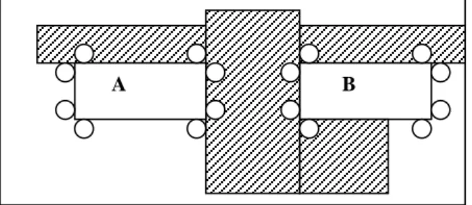
This idea is approximated using an eight points tightness heuristic, which is illustrated in Figure 2. For each candidate move, we look at the points that are immediately adjacent to
each corner of the candidate rectangle. That is, suppose a rectangle has the corners {(𝑥0, 𝑦0), (𝑥0, 𝑦1), (𝑥1, 𝑦1), (𝑥1, 𝑦0)}, we check whether the 8 corner adjacent points {(𝑥0, 𝑦0− δ ), ( 𝑥0− δ , 𝑦0), (𝑥0− δ , 𝑦1), (𝑥0, 𝑦1+ δ ) (𝑥1, 𝑦1+ δ), (𝑥1+ δ, 𝑦1), (𝑥1+ δ, 𝑦0),), (𝑥1, 𝑦0− δ),)} are occupied. The fitness of each move is then defined as the number of corner adjacent points that is not located in open space (that is, not in packed area, and not exceeding the container boundary). In Figure 2, the fitness of moves A and B are four and five respectively.
D. LFFT for Stock Cutting (LFFT-SC)
LFFT can be adapted quite easily for stock-cutting problems.
The idea is illustrated in Figure 3 as the LFFT-SC mechanism.
We start with a minimal container with base width w. The LFFT-PsP algorithm is applied repeatedly with increasing container height, until a packing solution is found.
Alternatively, for very large problem instances, the faster LFFT-IGE procedure can be used to replace LFFT-PsP (step 4 of Figure 3).
E. Computational Complexity of LFFT
The placement of a rectangle in each step of the algorithm will occupy one or more corners, and, at the same time, also generates a few new corners. Therefore, the number of corners at any time should be proportional to n, where n is the total number of rectangles, and the length of the move list in each step is bounded by O(q * n), where q is the parameter as mentioned above. In our implementation, the packed rectangles are stored using a k-d tree data structure [14], which provides a fast O(log n) region search operations. As a result, the complexities of LFFT-IGE and LFFT-PsP are O(qn2log n), and O(qn4log n) respectively.
III. MULTI-STAGE REDUCTION STRATEGY FOR AREA-MINIMIZATION PROBLEMS A. Multi-stage reduction Strategy
LFFT, with its Pseudo-packing-based algorithm, was originally a mechanism designed for the bounding-box packing problem. To adapt it for area minimization problems, where the problem spaces are much larger, we can utilize a multi-stage reduction approach, explained as follows. The idea is that, starting from a wide range of possible values of container widths, we incrementally reduce the number of candidate widths according to a multi-stage reduction schedule. Each stage would employ a successively more complex (and accurate) algorithm to cut down on the number of candidate widths, so that only the ones that deem most promising are retained. Finally, each of the remaining widths
A B
Fig. 2. The Tightness heuristics
Pseudo-packing-based Packing Algorithm (LFFT-PsP) Input: 1. A set of rectangles. 2. The parameter q.
1. Repeat the following steps (2 – 9) until all rectangles are successfully packed, or that there are no more legal moves.
2. Let L be the list of the remaining longest q rectangles that are not yet packed.
3. Generate an updated list M of (rectangle, corner) pairs, where rectangle is in L, and corner is a corner location that the current rectangle can be placed without overlapping. Each (rectangle, corner) pair constitutes a move.
4. For each move m=(r, c) in M
5. Pseudo-pack m by temporarily placing rectangle r at the corner c
6. Evaluate move m using the Iterated Greedy Evaluation Procedure (LFFT-IGE), and use the resulting packing density as the score of m.
7. Undo move m 8. End for-each
9. Select the move in M with the highest score and pack it permanently. Update L and M.
Iterated Greedy Evaluation Procedure (LFFT-IGE)
10. Repeat until all remaining rectangles have been pseudo-packed, or that no more move is possible 11. Let 𝑀′ be the updated list of remaining moves.
12. For each move 𝑚′ in 𝑀′, evaluate its fitness using a fast evaluation heuristics (e.g., the tightness heuristics).
13. Select the move in 𝑀′with the highest fitness values. Pseudo-pack this move.
14. End-Repeat
15. Compute the resulting packing density
16. Undo all pseudo-packed rectangles in steps 10-14.
Fig. 1. The LFFT Pseudo-Packing-based Packing Algorithm and the Iterated Greedy Evaluation Procedure
.
LFFT procedure for Stock-cutting (LFFT-SC) Input: 1. A set of rectangles. 2. Container width w.
Initialization:
1. Let rect_area be the sum of the areas of all rectangles 2. Let h = ⌈𝑟𝑒𝑐𝑡_𝑎𝑟𝑒𝑎 / 𝑤⌉
Procedure:
3. Repeat until all rectangles are successfully packed.
4. Execute LFFT-PsP or LFFT-IGE to pack the rectangles, with container width w and height h.
5. If all rectangles can be packed successfully 6. Quit.
7. else
8. Let h = ⌈ℎ × (1 + 𝛿)⌉
Fig. 3. Procedure for adapting LFFT for stock cutting
.
after reduction are packed using a stock-cutting mechanism (e.g., LFFT-SC) and the best solution is selected.
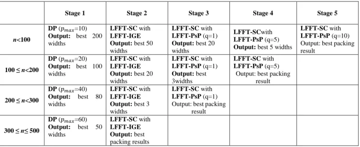
An example reduction schedule is depicted in Figure 4. In this example, the schedule to be followed is determined by the number of rectangles (n). In all cases, the first stage utilizes a dynamic programming (DP) algorithm for suggesting a promising set of candidate widths (discussed in the next subsection), which are then passed to the next stage.
Depending on n, the next few stages either employ LFFT-SC with LFFT-PsP, or LFFT-SC with the less complex LFFT-IGE algorithm. Different values for the parameter q are used in the various stages to keep the running time manageable. In each case, the rectangles are trial-packed using containers of each suggested width in turns, and the widths that produce the best results are kept. For example, given a problem with 150 rectangles. We first employ the DP procedure to produce a list of the 100 most promising width values (stage 1). For each of these widths, we employ LFFT-SC with LFFT-IGE to pack the rectangles. The 20 width values that produce the best results are passed to stage 3, which performs 20 rounds of packing using LFFT-SC with LFFT-PsP and with q=1. The best 3 results are then re-analyzed using LFFT-SC with LFFT-PsP, but this time using q=5 (which produces better results but the expected running time is 5 times as long than the previous stage for each problem instance). The best packing result is then reported. Note that this schedule has been tuned with a goal that the whole packing process can be completed in reasonable time using a single contemporary PC computer, after referencing the running time of a number of related approaches reported in the literature for common benchmark problems (see Section IV for details).
B. Dynamic programming method for 2D-CP problem reduction
For all problem size n, the first stage of the proposed reduction schedule relies on a dynamic programming (DP) procedure for reducing the initial set of possible width values into a more manageable set of promising widths for further evaluation. The DP procedure we use is adopted from an approach described by Bortfeldt in [6] for the Interval Subset Sum Problem (ISSP). The problem can be stated as follows.
Given a set of rectangles, and a maximum length 𝑝𝑚𝑎𝑥, we
want to determine the number of combinations of no more than 𝑝𝑚𝑎𝑥 rectangles whose widths add up to various values.
More specifically, we want to know the most frequently occurring sum of rectangle widths, for combinations of no more than 𝑝𝑚𝑎𝑥 rectangles. The idea is that those frequently occurring sum-of-widths should also serve as good indicators for promising container widths for the area minimization problem. A good explanation for an implementation of a dynamic programming procedure for ISSP problem is provided in [6], so we shall not repeat the details here. For now, it is sufficient to note that the abovementioned DP procedure has a worst case complexity of O(wmaxn2), where wmax is the largest possible sum-of-widths and n is the number of rectangles. In our implementation, the DP procedure finishes within one minute in all problem instances.
IV. EXPERIMENTS
We implemented the LFFT mechanism (LFFT-PsP, LFFT-IGE, LFFT-SC) as well as the DP procedure on a 3.2 GHz PC with 8 gigabytes memory. 4 The proposed method are tested using 33 publicly available 2D-CP problem instances, including nine well-known MCNC and GSRC benchmark problems, as well as 24 more recent RPAMP problem instances from [6]. Note that our focus is on medium to large problem sets with 50 or more rectangles. For this reason, several smaller MCNC and GSRC problems are not included (with the exception of ami33 and ami49, which are included due to their popularity in the 2-D packing literature).
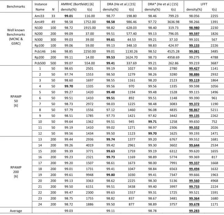
We compared our result with three of the state-of-the-art approaches at the time of writing, namely, the AMHRC results by Bortfeldt [6], and the DRA and DRA* results published recently by K. He et al. [15]. The results are given in Table 1, where the leading approaches are highlighted using bold fonts. We see that both LFFT and DRA performed very well for the MCNC and GSRC problems, with both approaches producing the best results in four instances, while AMHRC produced the best result in the remaining one problem. For the 24 new RPAMP problem instance, LFFT turns out to be far superior. Out of all 24 problems, LFFT is
4 Inter(R) Core(TM) i5-4460 3.20 GHz with 8.00 gigabytes RAM, running Windows 7.
Stage 1 Stage 2 Stage 3 Stage 4 Stage 5
n<100
DP (𝑝𝑚𝑎𝑥=10) Output: best 200 widths
LFFT-SC with LFFT-IGE Output: best 50 widths
LFFT-SC with LFFT-PsP (q=1) Output: best 20 widths
LFFT-SCwith LFFT-PsP (q=5) Output: best 5 widths
LFFT-SC with LFFT-PsP (q=10) Output: best packing result
100 ≤ n<200
DP (𝑝𝑚𝑎𝑥=20) Output: best 100 widths
LFFT-SC with LFFT-IGE Output: best 20 widths
LFFT-SC with LFFT-PsP (q=1) Output: best 3widths
LFFT-SC with LFFT-PsP (q=5)
Output: best packing result 200 ≤ n<300
DP (𝑝𝑚𝑎𝑥=40) Output: best 80 widths
LFFT-SC with LFFT-IGE Output: best 3 widths
LFFT-SC with LFFT-PsP (q=1) Output: best packing
result 300 ≤ n≤ 500
DP (𝑝𝑚𝑎𝑥=60) Output: best 50 widths
LFFT-SC with LFFT-IGE Output: best packing results
Fig. 4. A multiple-stage reduction schedule for area-minimization problems
able to improve on the currently best-known results in 15 cases (or 63% of the problems), while DRA is the second-best by leading in 6 of the problems (25%). The overall packing density of LFFT for all problem instances is also superior (99.3% for LFFT vs 99.1% for DRA vs 98.8%
for AMHRC), while the execution time is comparable. Note that LFFT also has a relatively smaller complexity than DRA.5 The detailed packing results for each problem instance can be viewed at the hyperlink included in following footnote.6
V. CONCLUSION
The 2D rectangular packing area-minimization problems (AM) are harder than traditional 2D packing problems due to their larger problem space. In this paper, we proposed a multi-stage reduction approach for AM problems by extending a mechanism called LFFT, which is a proven mechanism for 2D packing and stock-cutting. A dynamic programming procedure and a scaled-down version of LFFT are first employed according to a reduction schedule, which reduce the problem to a smaller set of more manageable stock cutting problem instances. One or more executions of LFFT then follow for producing the final packing results, while further reducing the number of candidate width values in each execution. This approach has been evaluated using publicly available problem instances and the results are encouraging, with the extended LFFT mechanism out-performing the currently best-known results in 63% of the case tests.
REFERENCES
[1] Lodi, A., Martello, S., & Vigo, D. (1999). Heuristic and metaheuristic approaches for a class of two-dimensional bin packing problems. INFORMS Journal on Computing, 11(4), 345-357.
[2] Wu, Y. L., Huang, W., Lau, S. C., Wong, C. K., & Young, G. H.
(2002). An effective quasi-human based heuristic for solving the rectangle packing problem. European Journal of Operational Research, 141(2), 341-358.
[3] Wu, Y. L., & Chan, C. K. (2005). On improved least flexibility first heuristics superior for packing and stock cutting problems.
In Stochastic Algorithms: Foundations and Applications (pp. 70-81).
Springer Berlin Heidelberg.
[4] Burke, E. K., Kendall, G., & Whitwell, G. (2004). A new placement heuristic for the orthogonal stock-cutting problem. Operations Research, 52(4), 655-671.
[5] Wetweerapong, J., & Remsungnen, T. (2010). Solving the Rectangular Packing Problem by a New Bottom-Left Placement Method Incorporated with a Multi-Start Local Search. Foundations of Computing and Decision Sciences, 35, 127-141.
[6] Bortfeldt, A. (2013). A reduction approach for solving the rectangle packing area minimization problem. European Journal of Operational Research, 224(3), 486-496.
[7] Wäscher, G., Haußner, H., & Schumann, H. (2007). An improved typology of cutting and packing problems. European Journal of Operational Research,183(3), 1109-1130.
[8] Burke, E. K., Kendall, G., & Whitwell, G. (2009). A simulated annealing enhancement of the best-fit heuristic for the orthogonal stock-cutting problem. INFORMS Journal on Computing, 21(3), 505-516.
5 The reported complexity for one execution of DRA, as reported in [15]
is O(n10). However, one must note that this is a worst case complexity, assuming there can be up to O(n3) action spaces at any instance. Their average case complexity should be around O(n8), assuming there are O(n) action spaces at any time. In comparison, the average case complexity for one execution of LFFT is O(n4 log n), also assuming there are O(n) valid moves at any time.
6 Available at:
https://drive.google.com/a/hsmc.edu.hk/file/d/0B0jDBeaFyEu-QzlFQUkwYlZkOFU/view?pref=2&pli=1
[9] Leung, S. C., Zhang, D., Zhou, C., & Wu, T. (2012). A hybrid simulated annealing metaheuristic algorithm for the two-dimensional knapsack packing problem. Computers & Operations Research, 39(1), 64-73.
[10] H. Zhou and J. Wang, ACG- adjacent constraint graph for general floorplans, ICCD 2004 pp 572-575
[11] Chen, M., & Huang, W. (2007). A two-level search algorithm for 2D rectangular packing problem. Computers & Industrial Engineering, 53, 123-136.
[12] Li, Y., Li, Y., & Zhou, M. (2011, December). A greedy algorithm for wire length optimization. In Electronics, Circuits and Systems (ICECS), 18th IEEE International Conference on (pp. 366-369), 2011 [13] K. He, W. Huang, and Y. Jin. "An efficient deterministic heuristic for
two-dimensional rectangular packing." Computers & Operations Research 39.7 (2012): 1355-1363.
[14] J.L. Bentley, Multidimensional binary search trees used for associative searching, Communication of ACM 18 (9) (1975) 509–517.
[15] K. He, P. Ji, and C. Li. "Dynamic reduction heuristics for the rectangle packing area minimization problem." European Journal of Operational Research 241.3 (2015): 674-685.
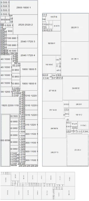
Fig. 5. Sample packing outputs: pcb146 (top left), Bortfeldt- 50-h07 (top right), Bortfeldt-50-h01 (Bottom)
TABLEI RESULTS OF COMPARISON
Benchmarks Instance AMRHC (Bortfeldt) [6] DRA (He et al.) [15] DRA* (He et al.) [15] LFFT Name N density(%) t(s) density(%) t(s) density(%) t(s) density(%) t(s)
Well known Benchmarks (MCNC &
GSRC)
Ami33 33 99.01 116.00 98.77 198.80 98.46 799.23 98.056 2255
Ami49 49 98.58 1752.00 98.58 986.46 97.72 3636.98 98.266 1391
N100 100 98.72 1915.00 98.82 628.03 98.40 319.73 98.980 2230
N200 200 99.09 37.00 99.51 577.40 99.13 796.05 99.597 1826
N300 300 99.03 39.00 99.61 44.53 99.21 37.10 99.101 567
Rp100 100 99.06 59.00 99.13 348.10 98.83 424.97 99.133 2226
Pcb146 146 98.85 2250.00 99.01 1130.26 98.52 4525.28 99.081 3485
Rp200 200 99.11 14.00 99.53 1624.70 98.73 4958.69 99.275 4788
Pcb500 500 99.07 554.00 99.41 337.69 99.21 262.86 99.219 3687
RPAMP 50 [6]
1 50 98.65 2501 99.19 1027 98.33 2780 99.427 1141
2 50 97.74 1553 98.50 1279 98.26 3280 98.886 2932
3 50 98.60 1697 98.55 1161 98.20 2123 99.119 1864
4 50 99.70 1335 99.56 970 99.56 1335 99.598 1056
5 50 99.27 1420 99.48 1194 99.48 1528 99.115 1496
6 50 99.51 1410 99.51 892 99.51 1148 99.390 961
7 50 98.73 2972 98.03 1225 98.48 3083 99.372 1190
8 50 97.79 1556 97.12 1460 96.08 4835 98.867 5211
9 50 98.51 1785 97.73 1421 97.82 3442 99.135 2262
10 50 99.64 1362 99.51 945 99.71 1258 99.650 752
11 50 99.19 1410 99.02 1271 98.97 2306 99.332 2026
12 50 99.56 1434 99.50 1123 99.70 1625 99.193 1471
RPAMP 200
[6]
13 200 99.44 2936 99.74 1377 99.20 6767 99.552 1681
14 200 99.26 4019 99.42 2961 99.30 3602 99.644 2534
15 200 99.39 3771 99.63 1759 99.19 6312 99.620 1655
16 200 99.23 2321 99.73 1169 98.89 5774 99.369 817
17 200 99.20 1507 98.61 1673 98.00 7991 99.337 1668
18 200 99.01 1731 99.41 1047 98.84 6563 99.494 1632
19 200 99.61 9948 99.80 1030 99.41 7347 99.666 1963
20 200 99.13 3363 98.62 2225 98.30 5136 99.560 4968
21 200 99.50 6151 99.51 3438 99.40 3997 99.733 2224
22 200 99.47 2300 99.63 1557 99.31 1725 99.521 1591
23 200 98.75 1755 98.82 837 98.67 3481 99.364 1680
24 200 98.72 1886 99.50 877 98.89 3757 99.678 1171
Average 99.03 99.11 98.78 99.283