Resilient Data Aggregation in Wireless Sensor Networks

(1)

ANANTHARAJU, SRINATH. Resilient Data Aggregation in Wireless Sensor Networks.

(Under the direction of Assistant Professor Peng Ning).

Sensor nodes are low-cost and low-power devices that are prone to node

compro-mises, communication failures and malfunctioning of sensing hardware. As a result, some

nodes may report outlying data values, introducing significant deviations in the aggregated

sensor readings. This thesis presents a practical resilient outlier detection technique to

fil-ter out the influence of the outlying data reported by faulty or compromised nodes. The

proposed outlier detection algorithm is based on event localization using minimum mean

squared error (MMSE) estimation combined with threshold-based consistency checking to

detect outliers. Data aggregation is one of the key techniques commonly used to develop

lightweight communication protocols applicable to wireless sensor networks. The proposed

approach handles localization of multiple events by grouping the sensor readings into

spa-tially correlated clusters and performing anevent-centricdetection of outliers. In the entire process of data aggregation, the outlier detection technique fits as a preprocessing stage for

reducing the effect of outliers on the aggregated result. Suitable extensions to the basic

outlier detection algorithm are proposed to effectively apply the algorithm to both

central-ized and decentralcentral-ized sensor network architectures. This thesis further includes studies

that test the effectiveness of the proposed approach, including the detection rate, the false

positive rate, degree of damage and the resilience to malicious readings introduced by the

attackers. The experimental results show that on average the proposed approach detects as

high as 80-90% of the outliers while resulting in 5-15% false positive rate when the network

consists of 40-45% outliers. The experiments also show that the extent of damage on the

aggregated result is below 50% due to the elimination of outliers before aggregation. Finally,

the resilient data aggregation process requires modest computational and memory

require-ments with zero communication overhead in the centralized case and about 20% overhead

(2)

by

Srinath Anantharaju

A thesis submitted to the Graduate Faculty of North Carolina State University

in partial satisfaction of the requirements for the Degree of

Master of Science

Department of Computer Science

Raleigh

2005

Approved By:

Dr. Douglas S. Reeves Dr. Ting Yu

Dr. Peng Ning

(3)

To my parents,

Sri. Kuruvadi Anantharaju, Smt. Chandrakala

and my brother,

(4)

Biography

Srinath Anantharaju was born on January 17, 1980 in Bangalore, India. He obtained his

Bachelor of Engineering Honors, BE(Hons) degree in Computer Science from Birla Institute

of Technology and Science (BITS), Pilani an autonomous university located in Rajasthan,

India in June 2002. After graduation, he worked with Insead Business School, France

as a Research Assistant from July 2002 to July 2003. He began his graduate studies in

Computer Science at North Carolina State University, Raleigh from August 2003. He has

acquired research internship experiences with ITC-IRST, Trento, Italy (Summer 2002),

Honeywell India Software Operations Pvt. Ltd. (January-June 2003) and IBM Zurich

Research Laboratory, Switzerland (Summer 2004). He started working with Prof. Peng

Ning at Cyber Defense Laboratory, NCSU from August 2004. He will be joining Google

Inc. in Mountain View, California after graduating with a Masters in Computer Science

(5)

Acknowledgements

First and foremost, I would like to thank my family: my father Sri. Kuruvadi Anantharaju,

my mother Smt. Chandrakala Anantharaju and my brother Sridhar Anantharaju for their

unconditional love and support throughout my life. I cannot describe in words what their

encouragement means to me and how thankful I am to them for all that they have done. I

am forever indebted to my parents and my brother, to whom I dedicate this thesis.

I would like to thank my advisor Dr. Peng Ning for his guidance and support

during my thesis research. His guidance and support were vital in completing this research

work. I learned a great deal about research in security and technical paper writing. I cannot

thank him enough for helping me realize my potential. I would like to thank Dr. Douglas

Reeves and Dr. Ting Yu for serving on my thesis advisory committee and providing me

with invaluable advice.

I would also like to thank Dr. Munindar Singh for his initial guidance in conducting

research and helping me bring out the best teaching potential as a supervisor for three

semesters. I thank Dr. Cliff Wang, Thomas Clouqueur, Dr. Kewal Saluja, Dr. Rob

Szewczyk, Dr. Joe Polastre, Mehmet Can Vuran, Dr. Caimu Tang and Dr. Sencun Zhu for

their support with valuable resources and enlightening discussions.

Last but certainly not the least, thanks to all my colleagues and friends at Cyber

Defense Laboratory: Donggang Liu, Dingbang Xu, Kun Sun, Jaideep Mahalati, Pratik

Shah, Pai Peng, Yan Zhai, Qing Zhang and Qinghua Zhang for useful comments. I would

also like to thank my friends Rithin Kumar Shetty, Mahesh Gajanan Aia and Naga Lakshmi

Mahali for their support during my research work.

Thanks to the Computer Science Department at North Carolina State University

(6)

List of Figures

2.1 Example of a centralized sensor network with a single aggregator (base station) . 8 2.2 Example of a distributed sensor network with intermediateaggregators . . . 9 2.3 The effect of distance to the light source on the photo sensor readings . . . 12 2.4 Cumulative distribution of the mean square errorζ2_{. Let}_k₌ ζ0

ǫ. . . 16

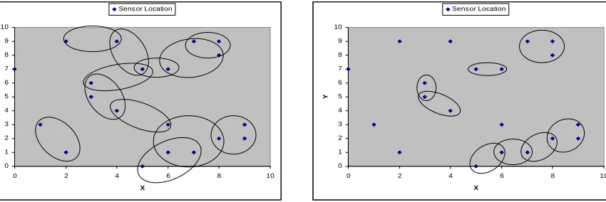
2.5 Spatial grouping of sensors in a 10m x 10m field(τc = 0.5) . . . 20

2.6 Spatial grouping of sensors in a 10m x 10m field (τc = 0.7) . . . 20

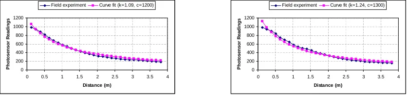
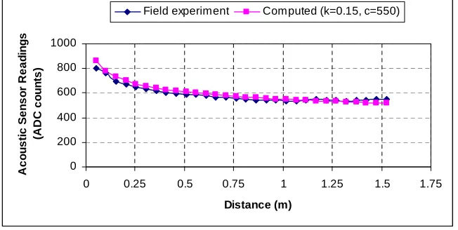
3.1 Determining the values of constantsk andc by fitting a suitable curve to the pho-tosensor readings obtained using field experiments . . . 31 3.2 The effect of the distance to the target on the acoustic sensor readings . . . 32 3.3 The effect of threshold on the outlier detection rate with a confidence interval of

90%. Letk=τ

ǫ. . . 33

3.4 The effect of threshold on the false positive rate with a confidence interval of 90%. Letk= τ

ǫ. . . 34

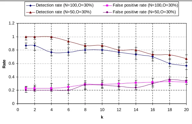
3.5 The effect of the local threshold on the outlier detection rate and the false positive rate withk= τl

ǫ and a confidence interval of 90% (Field size = 10m x 10m, outliers

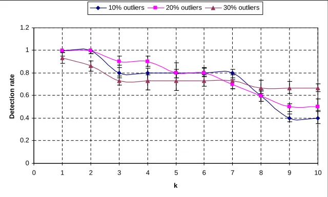
= 30%) . . . 35 3.6 The effect of the percentage of outliers on the detection rate with a confidence

interval of 90% . . . 36 3.7 The effect of the percentage of outliers on the false positive rate with a confidence

interval of 90% . . . 37 3.8 The effect of network density on the outlier detection rate and the false positive rate

with a confidence interval of 90% . . . 38 3.9 Comparison of the degree of damage on the MEDIAN before and after the outlier

elimination process (Network size = 400, Field size = 30m x 30m, Threshold = 10ǫ) 39 3.10 Comparison of the degree of damage on the AVERAGE before and after the outlier

elimination process with and without 5% trimming (Network size = 100, Field size = 10m x 10m, Threshold = 6ǫ) . . . 39 3.11 Effect of percentage of outliers on the outlier detection rate with a confidence interval

of 90% (Network size = 100, Field size = 10m x 10m, Threshold = 6ǫ) . . . 40 3.12 Effect of percentage of outliers on the false positive rate with a confidence interval

(9)

3.13 Effect of the local threshold on the detection rate and false positive rate in the centralized and distributed network scenarios withk= τl

ǫ and a confidence interval

of 90% (N = 50, Field size = 10m x 10m,τg = 4ǫ, Percentage of outliers = 30%) . 42

3.14 Physical layout of the sensor nodes, aggregators and the base station (N = 100, Aggregators = 10, Outliers = 30%) . . . 44 3.15 Comparison of the communication overhead as a function of the local threshold in

the centralized and distributed network scenarios. Letk= τl

ǫ (Percentage of outliers

= 30%) . . . 45 3.16 Comparison of the degree of damage as a function of the communication overhead

(10)

Chapter 1

Introduction

1.1 Background

Recent advances in wireless communications have enabled the development of tiny,

low-cost, low-power sensor nodes that are capable of sensing environment phenomena,

com-municating over short distances and processing small amounts of data. Sensor nodes mainly

use a broadcast communication paradigm and are limited in power, computational

capac-ities, and memory. For instance, the processing unit of a smart dust mote prototype is

a 7.3MHz microcontroller, with 8KB instruction flash memory, 4KB RAM and and a 916

MHz wireless transceiver capable of data transfer at 38.4 kbps with the radio range of 500

feet, and is powered by two AA batteries [23]. TinyOS operating system is used on this

processor, which has 3500 bytes OS code and 4500 bytes available space for application

programs.

A number of sensor nodes are deployed to monitor events of interest in the target

field, which form an ad hoc network to communicate sensor readings from the source to the

sink. Wireless sensor network applications are gaining popularity at a rapid rate due to

their applicability in sensing environmental phenomena, traffic monitoring, critical health

care monitoring and tracking of enemy battlefield operations. Sensors are usually deployed

in harsh environments that are prone to failures and node captures. Sensor nodes are highly

(11)

nodes vouching for an event in a particular region. The aim of redundant deployment is to

build reliable sensor network applications in a cost effective way.

The data collected by the sensor nodes is usually transmitted wirelessly to a

com-putationally powerful and sophisticated node called the base station. The base station is entrusted with the task of processing the received sensor data and derive meaningful

infor-mation representing the events in the target field. Sensor networks may contain intermediate

powerful nodes called aggregators deployed on the path between the sensor nodes and the base station. The aggregators collect data from a subset of the network, aggregate the data

using a suitable aggregation function and transmit the aggregated result to a higher level

aggregator or to the base station.

1.2 Motivation

Sensor nodes are not usually equipped with tamper-resistant hardware. As a

result, an attacker can take control of a sensor node by physically compromising it. Using

the compromised nodes, an attacker can easily manipulate the result of aggregation by

reporting malicious readings that introduce significant deviations in the aggregated result.

For example, a protocol that computes the average of sensor readings is insecure against

a single large reading introduced by an attacker. Current data aggregation techniques are

not designed with security in mind. Some of the popular aggregation functions such as

SUM, AVG, MIN, MAX and COUNT are shown to be insecure in [55]. Apart from node

compromises, an attacker can introduce significant deviations in the aggregated results by

creating fake events. For example, an adversary can artificially inflate a sensor reading by

holding a cigarette lighter in the vicinity of a heat sensor. Cryptographic authentication

mechanisms alone cannot solve this problem because an attacker may have access to valid

cryptographic keys via compromised nodes, and easily introduce deviating readings into

the network. Sensor nodes are also vulnerable to system faults that enable malfunctioning

sensors to report outlying data values. We denote all these deviating sensor readings as

outliers. It is of utmost importance to detect and eliminate the influence of the outliers on the aggregated result by designing a resilient aggregation scheme that can tolerate some

percentage of outliers.

(12)

certain general robust statistical techniques such as truncation, trimming and statistical

location estimators for eliminating outliers. However, these statistical techniques do not use any of the properties specific to sensor networks. These techniques can only mitigate

the problem of reducing the effect of deviating readings on the aggregated result. A direct

application of robust statistical techniques for resilient aggregation leads to problems

associ-ated with deciding the appropriate range of expected sensor readings, fixing the percentage

of highest and lowest readings to ignore, limitations of statistical location estimators such

as lower convergence rate, impractical for all but small datasets, inconsistency due to

ran-dom resampling techniques and unbounded influence in the case of high leverage points

as suggested in [43]. As a result, robust statistical techniques alone cannot guarantee

re-silient data aggregation. We believe that a complimentary approach that exploits some

of the properties specific to sensor networks can lead to an effective resilient aggregation

technique. Another important shortcoming of Wagner’s approach is that it does not handle

data aggregation in distributed network architectures. In a distributed sensor network, the

key challenge is that all the sensor readings required for aggregation may not be available

at a single node.

We believe that a practical data aggregation approach that incorporates some of

the properties specific to sensor network applications is a solution to all the above mentioned

shortcomings. In this thesis, we propose a resilient data aggregation technique based on

the attack-resistant minimum mean squared error estimation of the event location and the

threshold-based consistency checking among the sensor readings. Our approach detects and

eliminates outliers before proceeding with the aggregation of the sensor data. Unlike [55],

our method does not rely on the resilient properties of certain data aggregation functions and

works with any aggregation scheme, thus increasing its applicability in a variety of scenarios.

For example, our outlier detection algorithm can be incorporated into an acoustic sensor

network application irrespective of the aggregation function used. Our approach does not

rely on robust statistical techniques to eliminate the effect of outliers on the aggregated

result and guarantees detection rates as high as 80-90% while resulting in 5-15% false

positive rate.

Distributed network architectures are typically used to achieve energy efficient

information flow by aggregating the data values along the way from the source to the

sink. Our distributed resilient data aggregation algorithm compresses non-outlying sensor

(13)

parameters instead of the actual readings. The readings are regenerated at each of the

intermediate aggregators to determine the set of outliers that are transmitted to the higher

level aggregators. Finally, the base station executes the outlier detection algorithm to

eliminate the outliers before aggregating the sensor readings.

Sensor networks possess certain unique properties not commonly found in typical

distributed or centralized systems. Nodes physically located close to each other are likely

to report related data values, thus exhibiting spatial correlation properties. We make use of

this observation to group sensors into clusters and perform anevent-centricoutlier detection when multiple events are present in the target field.

1.3 Contributions

The scientific contributions of this thesis are fivefold:

• The thesis describes an outlier detection algorithm based on minimum mean square estimation (MMSE) for event localization. Using MMSE for determining the location

of the sensors is not novel, but estimating the location of the event based on the sensor

readings and the node localization information using MMSE is new.

• The thesis introduces a resilient outlier detection technique based on the distance-based event detection model for consistency checking among sensor readings with a

capability of handling multiple events in the target field.

• The thesis proposes an effective spatial correlation technique using spherical covari-ance model from geostatistics and maximal clique detection algorithm.

• The thesis describes a resilient data aggregation approach to detecting and eliminating outliers applicable to a distributed network architecture. To the best of our knowledge,

this work is the first on resilient data aggregation that can eliminate outlying sensor

readings before aggregation in a distributed network. The proposed approach can

handle outliers belonging to multiple clusters by combining outlier information at a

higher level for effective aggregation.

(14)

the resilience to node captures. We present a comparison of the performance of our

algorithm as applied to centralized and distributed network architectures.

1.4 Thesis Organization

The rest of this thesis is organized as follows: Chapter 2 describes in detail our

outlier detection process that combines the MMSE based event localization method while

checking for consistency among sensor reported readings. It outlines an algorithm for

group-ing the sensors into spatially correlated clusters in order to detect outliers when multiple

events are present in the target field. It also describes a distributed outlier detection

algo-rithm applicable to a network of distributed sensor nodes, with intermediate aggregators

deployed between the source and the sink. Chapter 3 presents an evaluation of the approach

using extensive simulations to demonstrate the effectiveness, including the detection rate,

the false positive rate and resilience to outliers. Chapter 4 describes the related work, and

(15)

Chapter 2

Resilient Data Aggregation

The damage caused by the compromised or faulty sensor nodes in the form of

outlying data values, on the aggregated result is tremendous. An attacker can introduce

significant deviations from the expected result if a non-resilient data aggregation function

is used for aggregation purposes. Computation of sum, average, minimum and maximum

are shown to be non-resilient [55]. In this thesis we do not concentrate on building resilient

aggregation operators but develop techniques to identify and eliminate outliers before

pro-ceeding with the task of data aggregation. We also highlight the resilient properties and

demonstrate the effectiveness of our outlier detection algorithm. In this chapter, we first

elucidate the assumptions we make throughout the thesis followed by a description of our

outlier detection process that can handle single and multiple events. We then describe our

outlier detection algorithms as applied to a centralized network consisting of a single base

station. We propose a distributed outlier detection algorithm applicable to a distributed

network scenario with low communication overheads and excellent scalable properties.

2.1 Assumptions

We assume sensor nodes are deployed with sufficient redundancy so that any two

sensors are within the sensing range of each other, redundantly monitoring an event that

(16)

because sensor nodes are usually deployed in large numbers to achieve sufficient reliability

in the absence of costly fault-tolerant hardware. Throughout this work we would be dealing

with static sensors. Static sensors are widely used in sensor network applications, including

acoustics, light sensing, magnetic field and harmful radiation detection, seismic vibration

sensing, tracking enemy tanks in a battlefield, temperature, pressure, surveillance and many

more. A sensor network application might make use of some computationally powerful

and sophisticated nodes called aggregators. The sensor readings are aggregated by the intermediate aggregators, as the data passes from the source (sensor node) to the sink

(base station). This results in energy efficient information flow in the network due to low

communication overheads.

In this work we assume the availability of the sensor location information either

hardcoded into each of the static sensors at the time of deployment or determined using one

of the localization techniques proposed in [44, 32, 11, 14, 49, 40]. Throughout this work we

consider an event-based system with one or more events occuring at any point in time and

the snapshot of sensor readings is analyzed for outliers. We also assume a simple model for

sensor measurement errors, where the measurement error is uniformly distributed between

−ǫand ǫ.

Sensor networks are used to monitor a variety of events in the target field. The

monitored events are either caused by environmental phenomena such as temperature and

pressure or due to visible objects such as enemy tanks in the battlefield. Our outlier

detection algorithm can only be applied to sensor applications that monitor the events

caused by visible entities, with a physical location in the field. We denote such events as

point events. Monitoring point events due to moving objects emitting light and magnetic radiations or the events causing vibrations fall under this category. It is not possible to

extend our approach to environment sensing applications like temperature or pressure. We

do not consider temporal correlation of the events. Our outlier detection algorithm is

executed periodically based on a snapshot of events monitored by the sensor nodes in the

target field.

We assume that all packets that are exchanged between the sensor nodes and the

aggregators are authenticated so that malicious data values introduced by the attackers

are easily filtered out without being considered for data aggregation. Some of the existing

practical approaches such as [28, 31] can be used for authenticating the messages exchanged

(17)

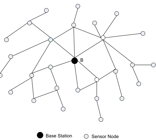
Base Station Sensor Node B

Figure 2.1: Example of a centralized sensor network with a single aggregator (base station)

packet authentication and TinyKeyMan [31] is a key management scheme for pairwise key

establishment in wireless sensor networks. We also assume that each node in the sensor

network is uniquely represented based on an identifier that is derived as a function of the

secret keying material specific to each of the nodes.

A sensor network usually consists of hundreds or thousands of tiny, cost,

low-power sensor nodes. We consider two kinds of sensor network architectures: a centralized architectureconsisting of a single base station acting as a sink, and adistributed architecture with intermediate aggregators. In the centralized case the base station is computationally

powerful and entrusted with the responsibility of aggregating the raw values reported by the

sensors. Figure 2.1 shows an example of a centralized network. A distributed architecture

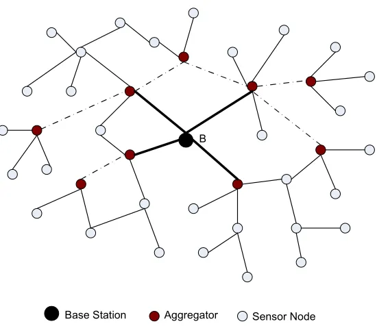
consists of several intermediate aggregators that are responsible for aggregating the data

from a subset of sensors and report the aggregated results either to a higher level aggregator

or to the base station. Figure 2.2 shows an example of a distributed architecture with

multiple aggregators, located on the path from the source to the sink. In a distributed

network, aggregating the data within the network prevents transmission of all the sensor

readings directly to the base station. This results in energy efficient information flow due

(18)

Base Station Sensor Node B

Aggregator

Figure 2.2: Example of a distributed sensor network with intermediateaggregators

Sensors deployed in a field could be heterogeneous in terms of sensing range,

com-munication range, battery power, computation and memory resources. The sensitivity of

the sensors to the event occuring at a particular distance could vary due to a drift caused

by age, decay, damage and accumulation of dust on the sensing hardware. There is a need

to identify and compensate the time-invariant systematic bias component of the error in

sensor measurements by employing certain calibration methods. We assume the existence

of a simple calibration technique used prior to deployment, so that sensors are calibrated to

provide consistent readings. An example calibration technique involves recording the sensor

measurements of all sensors placed at a fixed distance from the event and choosing one of

the sensors as a reference. The difference between the chosen sensor value and the rest of

the sensors are stored for compensating the errors before proceeding with outlier detection.

2.1.1 Attack model

Sensor nodes are deployed in hostile environments that are prone to node failures

and compromises. Using a compromised node, an attacker can induce highly deviating

(19)

Al-ternatively, if the nodes are protected by tamper-resistant packaging, then an attacker can

artificially inflate sensor readings by creating fake events. Outlying values are also an

out-come of failures in the sensing hardware. In all these cases it is highly desired to detect

these outlying values before proceeding with aggregating the sensor data.

We assume that an adversary’s capabilities in compromising sensor nodes or

arti-ficially inflating the readings are limited. Introducing significant deviations in each of the

sensor readings involve some cost for an attacker. Therefore an adversary can influence

only a limited number of sensor readings at a given point in time. We further assume that

the base station and intermediate aggregators are deployed fewer in number than regular

sensors, and it is possible to afford protecting them using highly tamper-resistant hardware.

These nodes remain trustworthy and difficult to be compromised by an adversary.

In this work, we do not consider the problem of colluding sensor nodes for the

purpose of introducing highly deviating readings into the network. In the case of a

distrib-uted network architecture, an attacker can compromise a local majority of the sensor nodes

and easily succeed in introducing outlying values into the aggregated result. However, a

redundant deployment of sensor nodes mitigates the effect of collusion to a great extent.

2.2 Resilient Outlier Detection: Single Event

The readings reported by the sensors correspond to events occuring in the field.

Depending on the sensing modality, the magnitude of a sensor reading for a point event is

influenced by the distance between the sensor node and the target causing the event. We

use an event detection model to estimate sensor readings based on the distance to the target

causing the event. Detecting and eliminating the influence of outliers is essential to avoid

deviating aggregated results representing an event in the target field. In this subsection,

we describe an outlier detection process adopted mainly from [49, 32]. However, our outlier

detection algorithm estimates the location of the event instead of node localization, using

minimum mean squared error (MMSE) estimation described in [49]. We use a

distance-based event detection model to estimate a sensor reading distance-based on the location of the

sensor from the estimated event location. Unlike [32], we compute the difference between

the actual and estimated sensor readings to check for threshold-based consistency among

(20)

The outlier detection algorithm described in this section works with a snapshot

of sensor readings representing a single event of interest in the field. However in a typical

sensor field multiple events can occur simultaneously. In the next section, we propose an

extension to our outlier detection algorithm that can handle multiple events by grouping

spatially correlated sensor readings.

2.2.1 Event Detection

Standard energy models for signal transmission is based on the fact that the energy

measured by a sensor i is a function of its distance di to the target object generating the

event. The strength of the signal emitted by a target object decays as a polynomial of

the distance between the sensor and the target [8]. The following equation generalizes this

notion of an energy model:

ri =c/(1 +di)k, (2.1)

where ri is the energy reading measured by the sensor, c is the maximum energy at the

target object called the energy constant, and k is a constant called the decay factor. The value of ktypically ranges from 2.0 to 5.0 depending on the environment as shown by field

experiments in [21].

We conducted field experiments using Mica2 motes to validate the above signal

strength equation. In our experiment, the target is a light emitting source and the

ex-perimental platform consists of a base station and a photo sensor. The sensor node is

programmed to sense the light from the target object and broadcast the detected signal

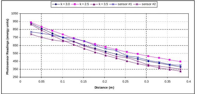
values. The base station is coded to receive the signals from the sensor node. Figure 2.3

shows the result of our experiments as a plot of photo sensor readings against the distance

of the light source from the sensor node. We used two different sensor nodes to record our

observations, and different sensors generated different readings for the same distance values.

For comparison purposes, we show the computed energy values forc= 1000 andk= 2.5,3.0

and 3.5 in figure 2.3. It can be seen that the energy readings reported by the sensor nodes

closely match the computed energy values fork= 3.0. Based on our field experiment results

and the suggestion made in [51] we use a value of k= 3.0 in all our simulations. The

rea-son for small deviations in our recorded observations could be attributed to the shadowing

effects and the sensitivity of the reading to the direction of the light falling on the photo

(21)

sensors for estimating the decay constant and the energy constant parameters in the event detection model. 250 350 450 550 650 750 850 950 1050

0 0.05 0.1 0.15 0.2 0.25 0.3 0.35 0.4

Distance (m )

P h o to s e n s o r R e a d in g s ( e n e rg y u n it s )

k = 3.0 k = 2.5 k = 3.5 sensor #1 sensor #2

Figure 2.3: The effect of distance to the light source on the photo sensor readings

As mentioned in section 2.1, one of our key assumptions is that we consider only

sensor applications that monitor point events caused by tangible entities characterized by

a physical location. It is not possible to extend our approach to environment sensing

applications like monitoring of temperature or pressure.

2.2.2 Event Localization Using MMSE

Our outlier detection process is based on the estimate of the event location using

the sensor node location information and a snapshot of sensor readings. The problem of

event localization is similar to node localization, and our method is adopted from the node

localization technique proposed in [49]. In the remainder of this subsection, we briefly

describe the event localization process using MMSE estimation.

The readings reported by the sensor nodes correspond to the events detected in

their vicinity. Sensor nodes are equipped with energy detectors that are typically used for

event detection. These detectors monitor signal energy over a period of time, and events

are recorded when the energy exceeds an application specific threshold [5]. We denote the

value reported by the sensori asvi.

As described earlier, the location of the sensor node is either hard-coded into the

nodes at the time of deployment, or securely estimated prior to the data aggregation phase.

(22)

triple hxi, yi, rii, where (xi, yi) is the location of sensor i, and ri is the value reported by

sensor i. Given a set of triples hxi, yi, rii representing sensor node locations and reported

values, we need to estimate the location of the event. The matrix solution to MMSE, as

described in [17], is used to estimate the location of the event monitored by a group of

sensors. The error of the measured distance between an unknown event and the ithsensor

detecting this event can be expressed as the difference between the measured distance and

the estimated distance, as indicated by equation 2.2. In 2.2 the estimated distance is derived

from equation 2.1.

f(xe, ye, c) = ((c/ri)1/k−1)−die (2.2)

Given a sufficient number of triples hxi, yi, rii, the location of the event can be computed

by taking the MMSE estimate of a system off(xe, ye, c) equations. If at least four triples

are available then it is possible to solve the system of equations for an estimate of the event

location (xe, ye) and the energy constantc.

2.2.3 The Algorithm

Our algorithm to detect outliers uses the method of threshold-based consistency

checking among sensor readings. Our approach is similar to the attack-resistant MMSE

location estimation described in [32]. In [32], Liu et. al use the difference between the

distance measured using the beacon signal and an estimate of the distance as a measure

of the error to check for consistency among a set of location references. However, in our

approach we use the difference between the actual sensor reading and the distance-based

estimated reading computed using equation 2.1. We check for consistency among the sensor

readings using a threshold value estimated by a procedure described in [32].

In the current approach, we consider all the sensor readings to estimate the location

of the event and the subsequent detection of outliers. The reading reported by a sensor

node that is located far away from the event is not influenced by the energy emitted by

the event. As a result, we can simply exclude these readings from the outlier detection

process. This reduces the number of sensor readings being considered for outlier detection

and a significant reduction in the computational complexity of the algorithm. If the sensor

readings are consistent, our outlier detection algorithm does not detect a distant non-outlier

as an outlier due to the low energy values reported by the sensor.

(23)

captures and failures. As a result, the event location estimated using the method described

in section 2.2.2 is prone to large influence by outliers. These outliers can easily influence

the event localization process and subsequently the data aggregation results computed by

the aggregator. In order to minimize this effect, we compute the mean square error ζ2 of the distance measurements based on the reported sensor readings and the estimated event

location. Given a set ofmtripleshxi, yi, riirepresenting sensor node locations and reported

values, we use MMSE to estimate the location of the event (xe, ye) and the energy constant

c. After that we compute the mean square error ζ2 _{of this location estimate using the}

following equation:

ζ2 =

m X

i=1

(ri−(c/(1 + p

(xe−xi)2+ (ye−yi)2)k)2

m (2.3)

We check for consistency among sensor readings by comparing the mean square

error against a given threshold value. All the inconsistent readings are branded as outliers

and not considered for data aggregation. Based on equation 2.1, we compute the difference

between the estimated reading, and the actual reading corresponding to a group of m

sensors, using equation 2.3. We check if a given set of sensor-specific triples hxi, yi, rii are τ-consistent w.r.t. the localization estimate obtained using MMSE as described in [32], whereτ-consistency among msensor readings is determined as follows:

ζ2 =

m X

i=1

(ri−c/(1 +die)k)2

m ≤τ

2 _(2.4)

The parametersτ and mare crucial in branding a group of sensors as outliers. In

what follows, we address the problem of estimating these parameters.

It is required to estimate a maximal subset of sensor readings that areτ-consistent so that the aggregated result is close to the actual result and only the genuine outliers are

discarded. An obvious method is to check all possible subsets starting from considering all

sensor readings until we obtain a subset that is found to beτ-consistent. In the worst case, this boils down to a powerset computation problem that is known to have an exponential

time solution. If a set containsmelements then the search space for computing the powerset

contains 2m elements. A sensor network with 20 nodes would require exploring all 220 = 1048576 subsets. Therefore, this algorithm is computationally expensive and does not scale

(24)

We make use of a suboptimal greedy strategy described in [32]. We start with

all sensor readings in the first round, compute the mean square error and check for τ -consistency. If they are τ-consistent then we conclude that there are no outliers in the given set of readings. If they are notτ-consistentthen we eliminate one triple such that the subset obtained produces the least mean square error as the input to the next round. The

algorithm continues until a τ-consistent subset of sensor readings is found. The number of rounds in this algorithm grows linearly with the number of nodes in the network. The

computational complexity is significantly reduced but the results obtained are suboptimal.

Estimating Threshold

It is difficult to propose a generic procedure to estimate an optimum value of the

threshold τ that is suitable to detect outliers in various sensor network applications. We

make use of the threshold estimation method described in [32]. For the sake of completeness,

we present a brief overview of the threshold estimation procedure. Further details can be

found in [32].

As suggested in section 2.1, we assume the availability of a simple measurement

error model, where the measurement error is uniformly distributed between−ǫand ǫ. De-termining an appropriate value of the threshold τ is dependent on the measurement error

model. The distribution of the mean square error ζ2 in the absence of malicious attacks is used to compute an appropriate value of the threshold. The measurement error

correspond-ing to a non-outlier triplehxi, yi, rii can be computed asei = (ri−c/(1 +die)k), where die

is the distance between the real location of the event (xe, ye) and the location of the sensor

node si. Using the lemma proposed in [32], we can obtain the probability distribution of

ζ2 _as_lim

m→∞F[ζ2≤ζ02] =φ(

mζ2 0−µ

′

σ′ ), where µ ′

= Σm i=1µi,σ

′

=qΣm

i=0σ2i, andφ(x) is the

probability of a standard normal random variable being less thanx. Assuming a uniform

dis-tribution of the measurement error between−ǫand ǫ, the mean and variance for anye2_i are

ǫ2

3 and 4ǫ

4

45 respectively. Substituting these values, we obtainF(ζ2 ≤(kǫ)2) =φ(

√

5m(3k2

−1)

2 ).

Using the probability distribution ofζ2obtained from the lemma, and the simulation results using the estimated event locations, we can determine an appropriate value ofτ.

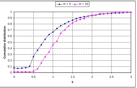
Figure 2.4 shows the probability distribution of the mean square errorζ2 _obtained

from two different simulations using sensors’ estimated locations. We use two different sets of

(25)

0 0.1 0.2 0.3 0.4 0.5 0.6 0.7 0.8 0.9 1

0 0.5 1 1.5 2 2.5 3

k C u m u la ti v e d is tr ib u ti o n

m = 5 m = 10

Figure 2.4: Cumulative distribution of the mean square errorζ2_{. Let}_k₌ζ0

ǫ.

and the other withm= 10 references. We can see that the cumulative distribution function

mimics an S-shaped curve. The figure gives a hint about the appropriate choice of the

thresholdτ. Specifically, the value of τ corresponding to a desired cumulative probability

is chosen for outlier detection. It is desirable to choose a threshold value corresponding

to a high cumulative probability (say 0.9). Figure 2.4 shows a threshold value ofτ = 1.9ǫ

achieves a probability of the mean square error greater than 0.9 observed in both the

simulated scenarios. This means more than 90% of the cases results in a mean square error

lesser than that computed using ζ0 = 1.9ǫ. A similar experiment can be conducted to

derive the actual distribution of the mean square error, and then determine the value of τ

accordingly.

We present the result of our experiments to demonstrate the effect of the threshold

values on the outlier detection rate and the false positive rate in section 3.3.

2.3 Resilient Outlier Detection: Multiple Events

The outlier detection scheme outlined in the previous chapter is designed with a

single target in mind. In the presence of multiple targets, the raw energy value detected

by a sensor is influenced by different targets to a different extent based on the distance

between the sensor and each of the targets. As a result, a simple application of our outlier

(26)

location estimation using MMSE and the consequent erratic detection of outliers. In this

subsection, we propose an extension to our outlier detection algorithm in order to handle

multiple events. We present a clustering technique to group the sensor readings into spatially

correlated clusters, and make use of these clusters to isolate sufficiently separated events

for outlier detection. This is the essence of ourevent-centricoutlier detection process when multiple events are present in the field.

2.3.1 Spatial Correlation

Typically sensor network applications require a dense deployment of sensor nodes

that are spatially close to each other for a reliable coverage of the region. The high network

density results in spatially proximal sensor observations that are highly correlated. The

extent of correlation increases with decreasing inter-sensor separation. In the remainder of

this subsection, we introduce a novel maximal cliques based approach to group spatially

correlated sensor readings for the purpose of outlier detection, in the presence of multiple

events.

As stated in section 2.1, we assume the availability of the sensor nodes location

information. Let us denote (xi, yi) as the 2-dimensionallocation of a sensor node si. The

distance between any two sensors si and sj, denoted bydij, can be computed easily with

the help of the available location information. The sensing range of a sensorsi, denoted as

Ri, varies from node to node in a network of heterogeneous sensors. With this information

in hand, we construct a graph of sensor nodes G(S, E) withS representing a set of sensor

nodes and E corresponding to a set of edges connecting sensor nodes based on inter-node

distances and the sensing ranges using the following condition.

ifdij < Ri anddij < Rj then

add an edge between sensors si and sj

end if

After constructing a graph of sensor nodes, we need a covariance measure to

quan-tify the spatial correlation property existing between any two sensor nodes. In what follows,

we discuss a simple covariance measure used in our approach followed by a description of the

(27)

The maximal cliques detection algorithm works with the pairwise correlation co-efficients

and a thresholdτc as the input, to group the sensors into spatially correlated clusters.

Covariance Measure

A covariance measure quantifies the spatial correlation property based on the

inter-node distance between any two sensor inter-nodes. Based on the covariance measure, sensor

readings are grouped into spatially correlated clusters. These clusters are used to generate

event-centric groupings specific to each event in the field. The outlier detection algorithm is then executed within each of these groupings for detecting outlying values.

Spatially varying phenomena are often modeled using Gaussian random fields,

specified by their mean function and covariance function. In [4], Berger et. al suggest four

standard families of covariance functions to model spatial correlation. One of these standard

families of covariance functions is borrowed from the field of geostatistics. Geostatistics is

a rapidly evolving branch of applied mathematics which originated in the mining industry.

It is now a popular technique in many fields of science and engineering where there is

a need to evaluate spatially or temporally correlated data [54]. Inspired by the field of

geostatistics, we choose spherical covariance model mainly due to its simplicity. Besides

simplicity, another motivation for choosing the spherical correlation model is its ability to

model continuous phenomena. Sensor nodes are typically equipped with energy detectors

which monitor signal energy in a time window and these energy values are consolidated into

a sensor reading using a method specific to the sensed phenomena. For example, discrete

events are reported by sensor nodes using a threshold based approach [5]. The spherical

covariance model is defined by the following equation:

ρij = 





1−3₂(dij

θ1) +

1 2(

dij

θ1 )

3 _{if 0}_≤_d

ij ≤θ1;

0 ifdij > θ1

(2.5)

and θ1>0.

In the above equation, ρij is the pairwise correlation coefficient that quantifies the spatial

correlation property existing between two sensors si and sj, separated by a distance dij

in the field. The parameter θ1 is called the range parameter and it indicates the range of

(28)

are uncorrelated. The range parameter is the maximal distance at which the volumes of influence of two spheres, representing sensor node ranges, can overlap and share information.

Therefore, in our simulations we useθ1as the average diameter of the sphere that represents

the sensing range of a typical sensor node. The covariance function is assumed to be

non-negative and decrease monotonically with the distance dij, having limiting values of 0 at

dij =∞ and of 1 at dij = 0; see [54] for a complete derivation of the spherical covariance

function.

Maximal Cliques Detection

Sensors can be coalesced into different groups such that nodes monitoring more

or less the same region are clustered into a clique. The idea behind this grouping is to

bring together sensors responsible for a particular event in a given area. Depending on the

sensing application, the sensor nodes in each clique are likely to report correlated values,

and the inconsistent data values within a clique are used to track outliers using our outlier

detection algorithm. It is well-known that finding maximal cliques in a given graph is

an NP-complete problem [9]. However, if the degree of a node is small, then finding all

maximal cliques a particular node belongs to is computationally feasible [52]. This is due

to the possibility of enumerating all maximal cliques in a reasonable amount of time.

In order to group the sensors into spatially correlated cliques, we make use of the

pairwise correlation coefficients computed using equation 2.5. An application dependent

cut-off value τc based on the pairwise correlation coefficients determines the level of similarity

necessary for clique membership. This cut-off value is a metric used by the maximal clique

detection algorithm to determine if two entities are spatially colocated.

The maximal cliques detection algorithm takes a matrix of pairwise correlation

coefficients corresponding to sensor pairs and an application dependent cut-off value τc.

Only the upper half of the correlation matrix values can be considered because of the

symmetric nature of correlation coefficients, i.e., ρij =ρji. Also self comparisons ρiican be

omitted to save some computational time and space. The output produced by the maximal

cliques detection algorithm consists of a list of all maximal cliques found with the given data

and a cutoff value. The sensors are coalesced into different groups based on this output.

Note that due to the possible overlap among cliques, a particular sensor node can be a part

(29)

0 1 2 3 4 5 6 7 8 9 10

0 2 4 6 8 10

X

Y

Sens or Location

Figure 2.5: Spatial grouping of sensors in a 10m x 10m field(τc = 0.5)

0 1 2 3 4 5 6 7 8 9 10

0 2 4 6 8 10

X

Y

Sens or Location

Figure 2.6: Spatial grouping of sensors in a 10m x 10m field (τc = 0.7)

The optimum cut-off value is decided by the node performing outlier detection, so

that the maximum possible nodes are clustered and any two nodes within a cluster are in

the sensing range of each other. We use a binary search process to determine the optimum

value of τc. Determination of τc starts with a cut-off value of τc = 1.0. At each step in

the binary search process, we test for the nodes being clustered and any two nodes within

a cluster to be in the sensing range of each other. The search process terminates when an

appropriate value ofτc is obtained such that the maximum possible nodes are clustered and

any two nodes within a given cluster are located in the sensing range of each other.

The effect of the cut-off value on the clique detection algorithm applied to a group

of 20 sensors in a field of size 10m x 10m is shown in figure 2.5 and figure 2.6. A comparison

of these two figures indicate that a lower cut-off value causes dense clustering of sensor nodes.

An increase in cluster density implies more sensor nodes vouching for events in a particular

geographical region, thus endorsing each other’s readings while checking for consistency. It

might seem to be a good idea to group all nodes into a single cluster by using a lowest

possible cut-off value, but this might result in a cluster containing non-correlated readings.

There is no point in grouping sensors widely separated from each other that do not report

spatially correlated readings. Figure 2.5 shows a grouping of almost all sensors into clusters

with a cut-off value of 0.5 while figure 2.6 indicates some sensors not grouped into any of

(30)

2.3.2 The Algorithm

In this section, we describe our event-centric outlier detection algorithm in order to handle multiple events present in the field. Counting the number of targets in the field

is presented as a peak counting problem in [5]. A non-outlying sensor node located closest

to an event is expected to report a reading that represents a peak in a two-dimensional

sensor field. In the past multiple events in the sensor monitored field has been studied as a

target tracking problem by correlating the sensor readings at different points of time. Our

approach is based on a snapshot of sensor readings representing a set of events in the target

field. As mentioned in section 2.1, we do not consider temporal correlation of the events.

The effect of multiple events on the energy values sensed by the nodes is dependent on the

application and the physical layout of the field. The key idea used in our algorithm is to

isolate sufficiently separated events by grouping the readings reported by the sensors close

to each of the events. When two or more events are closely located, then they are treated

as a single event in the process of detecting outliers.

We initially sort all the sensor readings representing a snapshot of the sensor field

and pick the sensorS reporting the highest reading. We then collect the readings reported

by the sensors belonging to all the spatially correlated clusters which the chosen sensor

S is a part. This gives an event-centric cluster of sensor readings. The outlier detection algorithm described in section 2.2, is applied within each of the event-centric clusters to identify the set of outliers. This is guaranteed to reduce the influence of multiple targets

on the outlier detection process except when multiple events are closely located. After the

first round of outlier detection, the algorithm proceeds by selecting the next highest reading

among the remaining nodes, and performing the outlier detection on the newly computed

event-centric cluster of sensor readings. The algorithm terminates when all the nodes are checked for outlyingness.

We often encounterevent-centricclusters with overlapping sensor nodes. A sensor reading in two or more clusters is influenced by the events occuring in each of the clusters. If

theevent-centric clusters arrive at inconsistent decisions about a given sensor measurement then we need a metric to resolve this inconsistency. We use the distance between location

of the sensor and the estimated event location as a metric to resolve the inconsistency

(31)

far away from the event. So, we consider only the decision of the event-centriccluster that contains an event located closer to the overlapping sensor node and ignore the remaining

decisions. If we consider an additive energy model to study the effect of multiple events on

a given sensor reading then such a reading is likely to be identified as an outlier by both

the clusters. However, detecting outliers in the presence of multiple events increases the

rate of false positives. We do not come across such a situation when the events are either

sufficiently separated or located close to each other.

Higher data values reported by a sensor indicates the occurence of an event in the

vicinity of the sensor. In a given set of sensor readings, we select the sensor reporting the

highest value as the closest point to the center of theevent-centriccluster within which we execute our outlier detection algorithm. Intuitively, this process assures a reduction in the

influence of multiple targets on the outlier detection process because each of the targets are

considered individually when the targets are sufficiently spread out. In the case of closely

located events, multiple events would be estimated as being produced by a single target

which again does not affect the detection of outliers to a great extent. When the algorithm

terminates all sensor readings are guaranteed to have passed through the outlier detection

process, being a part of the temporarily formedevent-centriccluster in atleast one round of the outlier elimination process. The end result is a set of sensor readings that have survived

all the outlier elimination rounds.

2.4 Distributed Outlier Detection

A sensor network usually consists of a large number of tiny, low-cost, low-power

sensor nodes deployed to monitor events of interest in the target field. These sensors are

highly limited in terms of their processing power, memory resources and battery life. Several

architectures have been proposed to save computation and communication overheads for

query processing in sensor networks [26, 34, 36]. The two most commonly used architectures

are: a centralized case with a powerful base station that collects and aggregates raw data reported by individual sensor nodes and adistributed casewith intermediate powerful and sophisticated nodes calledaggregatorsthat are deployed in small numbers. Each aggregator is responsible for aggregating raw data from a subset of sensor nodes within its range and

(32)

station. This is calledin-network aggregation. Figure 2.1 and figure 2.2 shows an example of a centralized and a distributed network architecture respectively.

The outlier detection algorithm described in the previous sections is applicable to

a simple centralized network scenario consisting of a set of sensor nodes reporting raw data

to a single aggregating node that could be the base station itself. In this section, we will

extend our approach to a distributed network setting comprised of a multi-hop network of

intermediate aggregators, each of which is responsible for aggregating the data reported by

a subset of sensors. A centralized network architecture is preferred when there is a need

to avoid the additional overheads associated with the establishment of the aggregation tree

that is required in the distributed setting. Additionally the base station is not required to

trust any other intermediate nodes in the network. But in a centralized scenario the base

station might be a bottle neck due to the processing of huge amounts of data collected

from a large network of sensor nodes. All the sensor readings are transmitted from the

source to the sink resulting in higher communication overheads. In a distributed network,

an aggregator shares the task of processing a subset of data values and performs in-network

data aggregation. Compressing a group of sensor readings into a single aggregated value

that is transmitted to the higher level aggregators leads to energy efficient information flow

in the network due to reduced communication costs.

2.4.1 The Algorithm

Figure 2.2 shows a multi-hop sensor network with multiple levels of aggregators

on the path from the sensor nodes to the base station. The aggregators apply our outlier

detection algorithm within each cluster to identify the set oflocal outliers before the data aggregation process. In this subsection, we present a distributed algorithm to build the

outlier detection hypotheses based on the information received from each of the lower-level

aggregators in the network hierarchy. Our aim is to reduce the number of false positives by

combining the outlier information from different clusters at the higher levels of aggregators.

We assume that all the aggregators in the sensor network are aware of sensor

locations. The location information could be hard coded into the nodes at the time of

deployment or determined as a part of the localization process. This is going to be a

one-time process since we are dealing with static sensors and aggregators. A higher level

(33)

the available location information and the transmission range of the nodes. This information

is used by the higher level aggregators in the distributed outlier detection process.

Each aggregatorAi collects raw energy readings from the sensors that are located

within the communication range, apply the outlier detection algorithm to estimate the

location of the event (xei, yei), the energy constant ci and the set of local outliers LOi

using a value of the local threshold τli. With in-network aggregation, an aggregator Ai is

expected to send the aggregated result to the higher level aggregator instead of forwarding

all the sensor readings. An advantage of using in-network aggregation is energy-efficient

information flow in a given network. However, in our approach the aggregators are not

required to send the aggregated result to the higher level aggregators but only forward

the estimated event location (xei, yei) and the energy constant ci along with a list of local

outliers LOi. For all those sensors not present in the set LOi, the higher level aggregator

recomputes the readings using equation 2.1, based on the information received from the

lower level aggregator.

The higher level aggregator Aj combines the set of computed readings with the

set of local outliers received and executes the outlier detection algorithm, described in

section 2.2. We obtain an estimate of the event location (xej, yej), the energy constantcj and

the set of local outliersLOj. The event location and the energy constant estimated by the

higher level aggregator is expected to be closer to the actual event location compared to the

values estimated by the lower level aggregators. This is due to more sensor readings being

available at the higher level and the effect of combining the readings from nodes belonging

to multiple clusters. The higher level aggregator Aj in turn forwards the estimated event

detection model parameters along with the set of local outliers to the upper level aggregators

in the network hierarchy. This process continues until the base station receives the model

parameters required to regenerate all the sensor readings. The base station determines

the final set of outliers O using the global threshold τg on the set of all computed sensor

readings. The outliers present in the setOare discarded and only the non-outlying readings

are considered for data aggregation. Thus the base station is able to compute anoutlier-free aggregated result in a distributed network scenario.

A sensor node can be physically located within the transmission range of more than

one aggregators. In such a case the higher level aggregator computes the sensor reading

based on the received event location estimate that is closest to the sensor node location. This

(34)

subsequent outlier detection process. A key factor influencing the outcome of our distributed

algorithm is the local threshold τl used by the lower level aggregators in the process of

deciding outliers. In section 3.3.2, we present the result of our simulation experiments to

study the effect of the local threshold τl on the distributed outlier detection process. A

stringent threshold value results in a bigger set of outliers required to be transmitted to

the higher level aggregators, thus adding to the communication overhead. On the contrary

a more relaxed τl gives a smaller set of outliers but at the cost of a higher rate of false

positives. The result of our simulations presented in section 3.4.6 and section 3.5.1 confirms

this observation.

A distributed network with intermediate aggregators scales well in the

manage-ment of a large network of sensor nodes. It reduces communication overheads by eliminating

the transmission of redundant information as the sensor readings move from the source to

the sink. It is a known fact that communication consumes more energy than

computa-tion. In-network data aggregation has been proposed as an effective technique to reduce

energy consumption due to communication by compressing the readings using a suitable

aggregation function by the intermediate aggregators. Our outlier detection process is built

on these ideas and makes an effective contribution to reduce communication overheads by

compressing the sensor readings into a distance-based energy model. The event detection

model parameters such as the estimated location of the event and the energy constant are

sufficient to re-generate the sensor readings at higher level aggregators based on the

avail-able sensor node location information. In section 3.5.1, we compare the communication

overhead incurred in both the centralized and distributed settings.

2.5 Limitations

In the previous sections, we have described our outlier detection schemes that

can handle single and multiple events. We also described the distributed outlier detection

applicable to distributed network architectures. In this section, we would like to address

some of the limitations of our outlier detection schemes. The limitations of our schemes are

mainly due to the assumptions we make in this work.

(35)

deploy-ment. An error introduced by the sensor node localization process can have a profound

impact on the detection of outliers. This is because we use the distance-based event

detection model to compute the estimated sensor reading based on the location of

the sensor. With a bunch of incorrectly estimated sensor readings, MMSE can give

sufficiently deviating estimate of the event location. This results in more and more

non-outliers being detected as outliers, thus increasing the rate of false positives.

• Sensor nodes can collude to introduce significant deviations in the aggregated result. We assume that in a given set of sensor readings considered for outlier detection, an

attacker is not in a position to compromise a majority of these readings. Suppose an

attacker is able to manipulate 60% of the sensor readings then we face a situation that

brands all the remaining 40% genuine non-outliers as outliers. Detecting and

elimi-nating these non-outliers can result in the final aggregation of completely malicious

sensor readings.

• Data aggregation schemes are highly dependent on the deployment of the sensor nodes in the target field. Consider a situation with a sparse deployment of sensor nodes.

In such a situation, the spatial correlation algorithm fails to cluster all the sensor

readings. As a result, we are forced to treat every sensor reading as a separate cluster

that does not help in theevent-centric detection of outliers when multiple events are present in the field. We also ignore the effect of obstacles that can have a significant

impact on the outlier detection process depending on the type of the event being

monitored. For example, a wall separating the light source (causing the event) and

the sensor node does not follow the pattern expected from the event detection model

described in section 2.2.1.

• Our outlier detection algorithm works on a snapshot of sensor readings. The frequency at which the snapshot is taken is dependent on the application. The outlier detection

process is carried out offline based on the collection of sensor readings. This method

based on a snapshot of sensor readings is not suitable for the real-time detection of

outliers due to the delay involved in the collection of the readings and the execution

of the outlier detection algorithm. Without time synchronization among the nodes, it

is difficult to take a snapshot of sensor readings such that all the readings represent

(36)

appropriate time synchronization algorithm and tag all the readings with a timestamp

when the event is detected.

• We assume that the aggregators are equipped with tamper-resistant hardware. As a result, they are completely trusted. This means an attacker cannot compromise

an aggregator to gain access to the cryptographic authentication keys shared with

each of the sensor nodes. However, aggregators are primary attack targets because

they process large amounts of sensor readings and compromising a single aggregator

can result in bringing down a significant portion of the network. So, an attacker

can use sophisticated techniques to compromise the aggregators in the network. A

compromised aggregator can either report malicious aggregation results or simply

drop the packets received from the sensors. Combining our outlier detection schemes

with techniques such as [12] that can detect compromised aggregators will result in a

(37)

Chapter 3

Evaluation

This chapter presents the result of our experiments to demonstrate the

perfor-mance of the outlier detection approach described in the previous chapter. We concentrate

on demonstrating the effectiveness of our approach using a simulation testbed consisting of

randomly deployed sensor nodes in a given target field. Our experiments do not take into

account the deployment of beacon nodes or some such special nodes that might be required

for estimating the location of the nodes. We also validate the event detection model with

the help of field experiments, using MICA2 motes equipped with acoustic and photo

sen-sors. While recording the results we take an average over multiple runs of the algorithm in

order to reduce the variations introduced by the choice of certain parameters like threshold,

sensing range and randomly generated event locations across simulation runs.

3.1 Evaluation Setup

The field experiments were carried out on MICA2 motes with acoustic and photo

sensors developed at UC Berkeley as a research platform for low-power wireless sensor

networks [27]. A MICA2 mote is equipped with a 7.3MHz microcontroller, 4KB RAM and

a 916 MHz wireless transceiver capable of data transfer at 38.4 kbps with the radio range of

500 feet, and is powered by two AA batteries [23]. We use Crossbow’s MTS310 sensor board

Resilient Data Aggregation in Wireless Sensor Networks

Contents

List of Figures

Chapter 1

Introduction

1.1

Background

1.2

Motivation

1.3

Contributions

1.4

Thesis Organization

Chapter 2

Resilient Data Aggregation

2.1

Assumptions

2.2

Resilient Outlier Detection: Single Event

2.3

Resilient Outlier Detection: Multiple Events

2.4

Distributed Outlier Detection

2.5

Limitations

Chapter 3

Evaluation

3.1

Evaluation Setup