Mitigation of Reverse Intermodulation Products at Colocated Base Stations

(1)

Mitigation of Reverse Intermodulation Products at

Colocated Base Stations

Shabbir Ahmed,

Student Member, IEEE,

and Mike Faulkner,

Member, IEEE

Abstract—In a colocated setting, large jamming signals from one transmitter can radiate into the antenna system of a second transmitter. The signals enter the second transmitter in the reverse direction and mix in the output stage of its power amplifier to produce intermodulation products. These ‘reverse’ intermodulation products get radiated from the antenna system and may fall on the victim receiver’s desired channel. The paper proposes an architecture that regenerates an estimate of the reverse intermodulation products using the fundamental jammer components and mitigates them in a baseband postdis-tortion cancellation circuit. A novel multiple-front-end receiver architecture is developed to overcome the high sample rate requirements if the jammers are well out of band. However, this leads to a frequency offset problem in the regenerated distortion estimate. Signal correlation is used to align the frequency, phase and amplitude of the distortion estimate with the interfering reverse intermodulation product. Simulations and theoretical analysis show the output signal-to-interference ratio (SIR) of the system is independent of the input SIR but dependent on the equivalent number of uncorrelated samples in the averaging block. A hardware prototype demonstrated a 16dB reduction of the interfering reverse intermodulation product.

Index Terms—Intermodulation products, postdistortion can-cellation, frequency offset correction, colocation, interference suppression, land mobile radio equipment, radio receivers, digital signal processing.

I. INTRODUCTION

C

OLOCATION of multiple transceivers of different wire-less standards on one common site increases the potential for mutual interference due to the close proximity of antennas. The problem is well recognised in the Defence industry where different air/land/marine vehicles have to accommodate many radio frequency (RF) platforms in a small area [1] [2] [3]. Lately, the rapid growth of the wireless industry has led to the deployment of a large number of base stations. Thus, the availability of new green field sites has been exhausted and service providers are now forced to share a common site. Although, sharing a common site reduces maintenance, rental, logistics and other costs, it causes interference challenges that need to be addressed.

In a co-located setting, base-station receivers have to receive weak desired signals in the presence of strong transmit signals (also called jamming signals in this paper) from neighbouring base-station transmitters; resulting in desensitization and the formation of intermodulation (IM) products. There are two major sources of IM products that may fall in the desired receive channel of the victim receiver [4].

The first are the IM products produced when high pow-ered jamming signals from the colocated transmitters mix

The authors are with the School of Engineering and Science, Victoria University, PO Box 14428, Melbourne, Victoria 8001, Australia (email: [email protected], [email protected]).

within the victim receiver’s front-end circuits (viz., low noise amplifier, mixer). The large jamming signal(s), regardless of their carrier frequencies, could also desensitize the receiver by forcing its circuits into saturation [5] [6]. Paper [7] addresses in detail such scenarios and proposes a feasible solution.

The second source of IM products are those radiated from the colocated transmitters themselves. In particular, the IM products that are generated when a high powered jamming signal from one transmitter radiates into the antenna system of a second transmitter and mixes in the output stage of its power amplifier (PA). These distortions are more precisely termed as ‘reverse’ IM products because of the manner in which they are produced and are specific to colocated scenarios. They may fall directly in the receive channel of a colocated victim receiver and cause interference. Further, the jammers need not necessarily be in-band, they could be out-of-band and still produce distortions within the victim receiver’s desired channel. In the case of out-of-band jammers both odd-order and even-order IM products could be of concern. Our paper here focuses on the elimination of these reverse IM products. The European Telecommunications Standards Institute (ETSI) standard [8] limits transmitter spurious output levels to −36dBm/0.1MHz below 1GHz, which is still too high to protect co-sited receivers. If co-sited receivers are present then there is a further reduction in the allowable spurious levels to −96dBm in the receive bands of other UMTS receivers on the same site. Unfortunately, it is not always possible to predict what future systems will be added to the site and so avoid the retrospective application of additional low insertion loss transmit filters, isolators or antenna placement strategies. The problem is even more difficult with the latest frequency agile cognitive technologies. It is the expense of retrofitting these systems we are trying to avoid.

Netcom [9] proposed an integrated frequency agile band-pass filter at the transmitter output to reject reverse signals entering the PA as well as stop any IM products produced from being transmitted. However, frequency agile high-Q filters with low insertion loss would be required to sufficiently attenuate the large transmitter signals, which, in some cases, have output powers of +47dBm (50W) [10]; a difficult and costly challenge. The scheme was targeted at defense applica-tions but is commercially unfeasible for many wireless service providers.

(2)

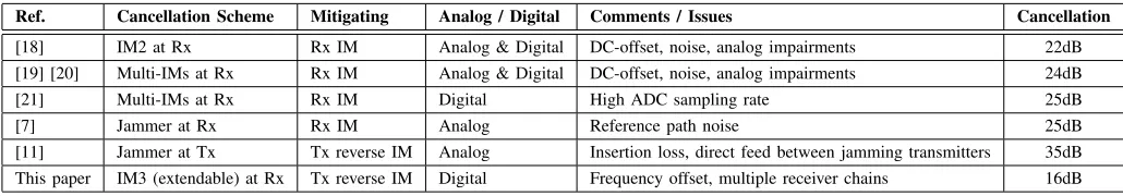
TABLE I

RELATEDIM DISTORTIONMITIGATIONSYSTEMS

Ref. Cancellation Scheme Mitigating Analog / Digital Comments / Issues Cancellation

[18] IM2 at Rx Rx IM Analog & Digital DC-offset, noise, analog impairments 22dB [19] [20] Multi-IMs at Rx Rx IM Analog & Digital DC-offset, noise, analog impairments 24dB [21] Multi-IMs at Rx Rx IM Digital High ADC sampling rate 25dB

[7] Jammer at Rx Rx IM Analog Reference path noise 25dB

[11] Jammer at Tx Tx reverse IM Analog Insertion loss, direct feed between jamming transmitters 35dB This paper IM3 (extendable) at Rx Tx reverse IM Digital Frequency offset, multiple receiver chains 16dB

insertion loss to the transmit path, and more importantly the victim receiver needs collaboration from the aggressor jammers for such transmit-end solutions. This is less likely in a multiple service provider scenario since it incurs further capital expenditures and the victim service provider is possibly a competitor. A solution is therefore required, that can be independently deployed by the victim receiver.

In [7], we used an adaptive cancellation system to reduce the jammers that hit the victim receiver front-end, thus, mitigating the formation of IM products. Likewise, authors of [3] removed them with tunable notch filters deployed at the victim receiver. However, removing the jammers at the victim receiver does not help mitigating the reverse IM products that are produced at the transmitter-end.

An alternate approach is to allow the distortion to occur and then cancel it at the victim receiver by regenerating an estimate of the distortion using the fundamental jammers. The concept, known as postdistortion, is the inverse of predistortion which is well researched and used in PA linearization. Predistortion systems can use either analog circuits or digital polynomial functions [12]- [17]. Similar circuits can be used to linearize receivers. The authors [18] and [19] used analog circuits to synthesize a distortion estimate for use in a digital adaptive postdistortion cancellation technique. Analogue squaring and cubing circuits often have inherent complexities such as direct feed-through, DC-offsets, temperature drifts and poor noise performance. On the other hand, digital polynomial functions have none of these problems; they are perfect (to within the quantization noise limit). Authors of [21] performed both distortion regeneration and distortion cancellation in the digital domain. The distortion corrupted desired signal along with the jammers are received in the RF front-end and downconverted to digital baseband. However, the demonstrated system is bandlimited by the ADC’s sampling rate and is unable to mitigate distortions produced by out-of-band jammers unless extremely large sampling rates are employed, making it both expensive and power hungry. The authors suggested the use of two parallel front-ends and ADC stages as a potential solution; one for the desired signal band and the other for blocker(s). This reduces the ADC resolution and sampling rate requirements. No further details were given.

The above postdistortion canceling schemes that target dis-tortions generated within the victim receiver are summarized in Table I (first four entries). The set of jammers that generate the distortion estimate in the regeneration circuits are exactly the same as those that generate the distortion products in

the receiver circuits. However, the dominant jammers causing the reverse IM products at the transmitter might not be the dominant jammers at the victim receiver. This sets the need for jammer selectivity for the regeneration circuits at the receiver. A full digital solution, similar to that of [21], would give the required flexibility for jammer selection, but the requirements of extremely high ADC sampling rates and processing power need to be addressed.

In this paper, we take advantage of the growing availability of low cost, wide-band software defined radios (SDRs) [22] [23] to extend the two-receiver solution suggested by [21] into a multi-receiver solution. We propose a novel postdis-tortion cancellation system using multiple SDR front-ends with reduced ADC sampling rate. As seen in Fig. 1, the primary SDR front-end (Rx0) receives the corrupt desired signal and converts it to digital baseband (y). The auxiliary SDR front-ends (Rx1,Rx2,..) are each tunned to a jamming signal that contributes to the interfering reverse IM distortion. These signals are also converted to digital baseband where they are described by their complex envelope representation (a,b,..). The fundamental jamming signals are processed in a nonlinear function to produce an estimate uˆ of the required reverse distortion product u. This is then subtracted form the primary received signal after appropriate gain and phase scaling. This effectively eases the spurious requirements for transmitter reverse intermodulation.

The structure of the nonlinear function depends on the distortion source, which can be from within the victim receiver

Rx1

Rx2

Rx0

NONLINEAR POLYNOMIAL

FUNCTION

+

_OUTPUT

FIR FILTER

ANALOG DIGITAL

PRIMARY FRONT-END

A

U

X

IL

IA

R

Y

F

R

O

N

T

-E

N

D

S

y=s+u a b

u

s

NONLINEAR POLYNOMIAL

FUNCTION

FIR FILTER

+

(3)

or from outside such as from passive IM distortion from poor connections or reverse intermodulation as discussed here. Even and odd order harmonics as well as multi-signal IM products can be synthesised using a polynomial function.

The scheme relies on the exact match in amplitude, phase and frequency of the distortion estimate uˆwith the distortion u in the received signal y. This can only be achieved if the frequency of the jamming signals are known. In practice, this assumption might not be valid, and even if the fre-quencies are known (e.g., from database look-up), component tolerances, aging and temperature drifts in the transceiver reference crystals produce unknown frequency offsets. If the jammer modulation is known the offset can be estimated using coherent detection. For example, carrier frequency offset [24] correction using pilots, cyclic prefix and signal statistics is well known for OFDM signals [25]- [27].

The solution proposed here does not require knowledge of these offsets or knowledge of the jamming signals’ mod-ulation. No spectral or time domain information about the jammers is assumed. However what is assumed, is the jammers are large and can be identified by a scanning receiver using simple energy detection. The frequency estimates are therefore very coarse and must be corrected as part of the distortion synthesis process. A novel two part frequency correction technique is described in this paper. It involves a combination of FFT and signal correlation to correct the frequency offset in the synthesized distortion.

Section II discusses a colocated base station model and the reverse IM products that cause interference. Section III de-scribes the novel distortion synthesis technique with frequency correction and the proposed postdistortion cancellation archi-tecture. Section IV characterizes the cancellation system using simulations and mathematical analysis. Section V presents a practical prototype of the cancellation system, measurements and results. Finally, section VI is the conclusion.

II. REVERSEINTERMODULATIONPRODUCTS

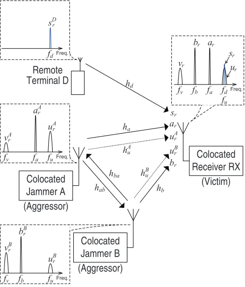
A model of three colocated base stations along with a remote terminal is shown in Fig. 2. Terminal D transmits the desired signal sD

r(t)1 over channel gainhd(t)to base station receiver RX. The spectrum of the output at terminal D shows the desired signalsD

r(t)at frequency channel fd. A high powered signal bB

r(t) from jammer B propagates through a channel gain of hba into the colocated power amplifier of jammer A and produces reverse third-order in-termodulation (IM3) productsuA

r(t)andvAr(t); withuAr(t)at fu, overlapping receiver RX’s desired channel frequencyfd, andvA

r(t)is at frequencyfv, given as follows,

fu= 2fa−fb (1)

fv= 2fb−fa (2)

where fa and fb are the transmit frequencies of aAr(t) and bBr(t) respectively. The IM3 products uAr(t) and vrA(t) are

1_Radio _frequency _signals _have _the _subscript _‘r’. _sD r(t) =

Re[sD(t)ej2πfdt]_{, where}_sD₍_t₎_{is the complex envelope.}

Colocated Jammer B (Aggressor) Colocated

Jammer A (Aggressor)

ha

hba hAu

hab hb

hd

hBu Remote

Terminal D

(Victim) Colocated Receiver RX br

uBr ar uAr sr

Freq.

br ar

vr _ur

sr

fd fa fb fv

fu

Freq.

aAr

uAr vAr

fu fa fv

Freq.

sDr

fd

Freq.

bBr

vBr

uBr

fu fb fv

Fig. 2. Colocated base station transceivers.

radiated from jammer A along with its own transmission. Spectrum A shows the output at jammer A.

Similarly, signal aA_r(t) from jammer A propagates over a channel gain of hab to generate reverse IM3 products uBr(t) and vBr(t) at jammer B. Spectrum B shows the output at jammer B.

Spectrum RX shows the signals vr(t), br(t), ar(t), ur(t) and dr(t) received at receiver RX after propagating through their respective channel gains. Reverse IM3 productvr(t)does not affect desired channelfd and is not of concern.

Large transmit signals ar(t) and br(t) could be of con-siderable concern if they exceed the dynamic range levels of receiver RX as discussed in [7]. However, in this paper, we consider them to be within receiver RX’s dynamic range and so do not contribute to the distortions within the receiver’s front-end.

Reverse IM3 product ur(t) falls directly on to the desired signal channelfdand causes interference for receiver RX. The IM3 productur(t)has two componentsuAr(t)anduBr(t)given by,

ur(t) = Re [(

hA_uuA(t) +hB_uuB(t))ej2πfut] ₍₃₎

where hA

u and hBu are the respective channel gains through which uA_r(t) and uB_r(t) propagate to receiver RX (Note: These gains are different fromha andhb because they are at different carrier frequencies);uA(t)anduB(t)are the complex envelopes.

The IM3 product uAr(t)is linearly affected by the channel gainhba, its magnitude is given as follows,

(4)

where gA

3 is the cubic distortion coefficient of jammer A’s power amplifier and is related to its output IP3 [6]. However, the magnitude of the IM3 productuB

r(t)depends on the square of the channel gainhab, as given below,

|uB(t)|=g3B|hab|2|aA(t)|2|bB(t)| (5)

where gB

3 is the cubic distortion coefficient of jammer B’s power amplifier. If both transmitter amplifiers are similar then the distortion coefficients gA

3 ∼ gB3. Thus, uBr(t) is usually very small and is considered negligible throughout this paper. A point to note, although the channel gain hd(t) is time varying, the other gains shown in Fig. 2,ha,hAu,hb,hBu,hba and hab are all considered to be quasi-static given the close proximities and fixed nature of the colocated antennas A, B and C.

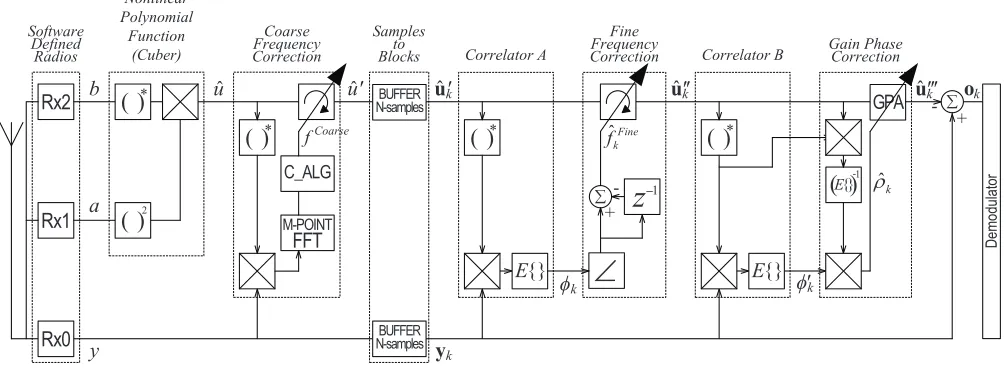
III. PROPOSEDARCHITECTURE ANDDIGITALSIGNAL

PROCESSING

The proposed architecture (Fig. 3) has an antenna feeding three SDR front-ends and a common DSP that synthesizes the interfering reverse IM3 product and removes it from the contaminated desired signal before the demodulator.

If the cancellation is to be effective the synthesized dis-tortion must have the correct amplitude, phase, timing and frequency. In this work timing accuracy is obtained by using the same sampling clock for all three receivers. Frequency locking is obtained using a correction algorithm and gain-phase correction is obtained by adaptive adjustment.

The sample rates have to be reasonably high because of frequency offsets and the bandwidth expansion that occurs on the nonlinear jamming signals. For example, the distortionur has a bandwidth of twice the bandwidth of the arsignal plus the bandwidth of thebrsignal. A large over sampling rate will handle most contingencies as well as give reasonable timing fidelity in the cancellation. Note, the sample rate is still much less than a single wideband receiver covering all jamming and desired signals.

The next subsections describe the major modules in the system.

A. Multiple Receivers

The victim receiver has multiple independently tuned RF front-ends. The primary receiver front-end Rx0 is tuned to receive at the desired signal frequency fd. It receives the desired signal sr(t) along with the interfering reverse IM3 productur(t). The received signal,

yr(t) =sr(t) +ur(t) (6)

where,

sr(t) = Re [

hd(t)sD(t)ej2πfdt ]

(7)

withsD₍_t₎_{being the complex envelope of} _sD

r(t), and,

ur(t) = Re [

g3AhAu hba{bB(t)}∗{aA(t)}2ej2π(2fa−fb)t ]

. (8) with aA₍_t₎_and_bB₍_t₎ _{being the complex envelopes of}_aA

r(t) andbB

r(t)respectively and{bB(t)}∗is the conjugate ofbB(t).

As discussed the non-linear IM3 products have expanded bandwidths and can cover many channels. The center fre-quency ofur(t)could therefore have a frequency offset∆fu of more than one channel fromfd(i.e.2fa−fb=fd+ ∆fu) and still cause interference to sr(t). Thus, ur(t) could be rewritten and expressed as follows,

ur(t) = Re [

g3Ah A

u hba{bB(t)}∗{aA(t)}2ej2π(fd+∆fu)t ]

. (9) The complex envelope of the received signal yr(t) is y(t) at receiver Rx0’s operating frequency fd. After sampling and analog-to-digital conversion the digital baseband signal is given by,

yn=sn+un (10)

wheresn is the desired signal component,

sn=hd,nsDn (11)

andun is the IM3 distortion component,

un=gu{bBn}∗{a A n}

2_ej2π∆fun/fs ₍₁₂₎

with2 _g

u =g3AhAu hba, and fs is the sampling frequency of the software defined radios.

The auxiliary receiver front-ends Rx1 and Rx2 scan for the out-of-band jammers ar(t) and br(t) respectively. These jammers are the fundamental components of the interfering IM3 product ur(t) and can be used to digitally synthesize the IM3 product at baseband. A relatively simple energy detection technique could be used to scan for the high powered jammers, since, an exact lock onto their carrier frequencies is not necessary. As such, the carrier frequencies f_a′ and f_b′ of their respective receiver front-ends Rx1 and Rx2 are at certain frequency offsets∆fa and∆fb from the jammer frequencies fa andfb, given as follows,

fa =fa′+ ∆fa (13)

fb=fb′+ ∆fb. (14)

The following are the received signals at Rx1 and Rx2 respectively in terms of the complex envelope components of the jammers,

ar(t) = Re [

haaA(t)ej2π(f ′ a+∆fa)t

]

(15)

br(t) = Re [

hbbB(t)ej2π(f ′ b+∆fb)t

]

(16)

which at digital baseband are as follows,

an=haaAne

j2π∆fan/fs ₍₁₇₎

bn=hbbBne

j2π∆fbn/fs_. ₍₁₈₎

The aim is to use these baseband jammer componentsan and bn to synthesize a duplicate of the received distortionun and remove it fromyn.

2_{Assumes that} _uB

r(t) is negligible compared to uAr(t). If not, due to amplifier differences, then the two distortion terms must be added giving

gu=g₃AhAuhba+gB3h

(5)

a b

Rx2

Rx1 Software

Defined Radios

Nonlinear Polynomial

Function (Cuber)

Coarse Frequency Correction

C_ALG

M-POINT FFT

+

-BUFFER N-samples

{}

E

( )

-1

GPA Fine

Frequency

Correction Correlator B Gain Phase Correction

+

-Rx0

k u

y yk

Samples to Blocks

u'

f Coarse

D

em

od

ul

at

or

( )

*

{}

E

{}

E

!

1

z

Correlator A

( )

*

( )

*

BUFFER N-samples

k '

k

o

ˆ_k

"

ˆFine k

f

u''k

u'k u'''k

( )

*

( )

2

Fig. 3. Proposed DSP.

B. Nonlinear Polynomial Function: Cuber

The cuber module, as shown in Fig. 3, starts the synthe-sization process. It produces a sample of the required IM3 distortion by taking an andbn as inputs, conjugating bn and then multiplying with the square of an to give,

ˆ

un=b∗na 2

n =gˆu{bBn}∗{a A n}

2_ej2π∆fˆun/fs ₍₁₉₎

whereguˆ=h∗bh2a and∆fuˆ= (2∆fa−∆fb).

A comparison between Equations (12) and (19) shows that the synthesization process would further require a frequency offset∆f correction such that,

∆fuˆ−∆f = ∆fu (20)

and a gain-phase correction ρsuch that,

ρguˆ=gu. (21)

Hence, un is given as follows,

un=ρuˆne−j2π∆f n/fs (22)

andyn can be reformatted as,

yn=sn+ρuˆne−j2π∆f n/fs. (23)

Further, the frequency tuning is a two part process. Whereuˆ is rotated for a coarse correction offCoarse _{and then tracked} in blocks and finely tuned byfF ine_{, i.e.,}

∆f =fCoarse+fF ine. (24)

C. Coarse Frequency Correction

To do coarse frequency correction we must first find the distortion signal uˆ withiny. To do this we use correlation.

Φ =E{uˆ∗_nyn} (25)

where E{·} is the expectation operator. Substituting for yn from (23) gives

Φ =E{uˆ∗_nsn}+E {

ρuˆ∗_nuˆne−j2π∆f n/fs }

. (26)

The first term is zero since ˆun is uncorrelated to sn. The product ofuˆ∗_nuˆnis always real and averaging gives its power. However, the frequency offset term ej2π∆f n/fs _{rotates the}

products and their average will tend to zero since most products would be balanced out with another product 180◦ out of phase. Thus, a second rotator is needed to reverse the frequency offset rotation prior to averaging. The FFT provides a bank of such rotators all rotating at different frequencies. It also provides the summation function for the averaging, and hence, it gives,

Φ(l) = M∑−1

n=0

{

ˆ

u_n∗sn+ρuˆ∗nuˆne−j2π∆f n/fs }

e−j2πln M,

l= 0,1, ..., M−1. (27) The correction algorithm C ALG usesΦ(l)to find the highest power binlmaxin theM-point FFT, i.e.,lmax= arg max

l

Φ(l).

Which givesfCoarse _{as follows,}

fCoarse=δMlmax (28)

where the frequency resolution isδM =fs/M. Large values of M are preferred in order to get an accurate frequency estimate as well as to minimize the noise contribution caused by the desired signal in the first term of (27).

Finally, the rotator in the coarse frequency correction mod-ule is set to correctuˆn by frequencyfCoarse such that,

ˆ

u′_n= ˆune−j2πf

Coarse_n/f

s_. ₍₂₉₎

The correction is only accurate within half a bin size δM/2. The small difference in rotation left between uˆ′_n and un in yn is then adjusted by the fine frequency correction module. Generally, coarse frequency estimation is only performed once at switch ON.

D. Fine Frequency Correction

The stream of samples uˆ′_n and yn is now buffered into blocks ofN-samples, thek-th block is defined below,

ˆ

u′_k=

[

ˆ

u′₀_,k uˆ′₁_,k ... ˆu′₍_N₋₁₎_,k ]T

(6)

yk = [

y0,k y1,k ... y(N−1),k ]T

. (31)

The blocks uˆ′_k andyk are then fed as inputs to correlator A. Correlator A evaluates the correlation (ϕk) ofˆu′k withyk,

ϕk =E{uˆ′∗n,kyn,k} ≈ (

ˆ

u′H_kyk

)

/N (32)

and forwards it to the fine frequency correction module. The parameter of interest is the phase of ϕk (̸ ϕk).

It is to be noted that yk has an IM3 distortion component uk and a desired signal componentsk, i.e.,yk =uk+sk. The aim is to alignû′_k’s frequency rotation withuk.E{uˆ′∗_n,kyn,k} calculates the average of all the angle differences between each sample ofuˆ′_k anduk. Hence,̸ ϕk holds the relative angle of the block û′_k to uk. And ̸ ϕk−1 holds the relative angle of the previous block û′_k₋₁ touk₋1. The difference in the two angles,

∆̸ ϕ≠ ϕk−̸ ϕk−1 (33)

gives the extra phase rotation that uˆ′_k obtains due to the fine frequency offset overN-samples. The fine frequency estimate then becomes,

ˆ

f_kF ine = ∆̸ ϕ fs/2πN. (34)

The rotator uses fˆ_kF ine to back rotate ˆu′_k with ∆̸ ϕ/N radians/sample over the block.

ˆ

u′′_n,k= ˆu′_n,ke−j2πfˆkF inen/fs_. ₍₃₅₎

This tunes uˆ′′_k to the same frequency as uk inyk.

E. Gain-Phase Correction

We use Bussgang’s theory [28] to identify the coefficient estimateρˆk which is the amount ofˆu′′k inyk, i.e.,

ˆ ρk=

E{uˆ′′∗_n,kyn,k}

E{uˆ′′∗_n,kuˆ′′_n,k} ≈

( ˆ

u′′H_kyk

) (

ˆ

u′′H_kˆu′′_k

). (36)

Further, ˆu′′′_k = ˆρkˆu′′k is subtracted from yk to give us the desired signal sk which forms the input to the radio demodulator.

F. Desired Signal Demodulation

The received signal yk is essentially intact/unaltered until the distortion estimate uˆ′′′_k gets subtracted at the input to the demodulator. Therefore, no modifications (e.g., frequency offset and gain-phase adjustment) are imposed on the desired signal sk. A standard receiver demodulator can be used. The demodulator would do the normal receiver functions of time synchronization, frequency synchronization, channel estimation and demodulation. Note, frequency synchronization here centers the desired signal modulation to DC. There is no relation between this and the frequency correction applied to the distortion estimate.

IV. SIMULATIONS ANDANALYSIS

In practice, a certain level of interferencezk remain at the output of the system. Thus at the canceler outputok becomes,

ok=yk−uˆ′′′k =sk+zk. (37)

This section identifies the different sources of interference that cumulate to give zk at the output. The investigation works backward from the canceler output to isolate and identify each of the interference sources.

A. Buffer/Data Processing Block SizeN

First, under investigation is the gain-phase correction mod-ule along with its correlator B that process data in blocks of N-samples; the preceding fine and coarse frequency correction modules are perfectly adjusted. Substituting forykin equation (36), we have,

ˆ ρk =ρ+

E{uˆ′′∗_n,ksn,k}

E{uˆ′′∗_n,kuˆ′′_n,k}, (38)

the latter term is zero, but, when the expectation takes the form of an average overNs uncorrelated samples, the output approximates a normal distribution,

ˆ ρk =N

{ ρ,σ

2 sσ2uˆ Nsσ_u4_ˆ

}

(39)

where the desired signal power E{|sn,k|2} = σs2, and the distortion estimate powerE{|uˆn,k|2}=σu2ˆ. Simplifying (39), we have,

ˆ ρk =N

{ ρ, σ

2 s Nsσu2ˆ

}

(40)

where the first term is the mean and the second term is the variance of a normal distribution. Since, the signals are over sampled we approximate Ns= ηN /OSR whereOSR is the over-sampling rate of the desired signal and equal to fs/bandwidth of s. The factor η is dependent on the modulation parameters of the signals a, b and s. We show in appendix A, η = (3/2)2 _{when all three fundamental} signals are Gaussian in nature and have a rectangular spectrum. Substitutinguˆ′′′_k in (37) withρˆkuˆ′′k, we have,

ok=N

{

sk,

σ2 sσu2ˆ Nsσ2ˆu

}

(41)

which is further simplified to give,

ok=N

{

sk,

σ2 s Ns

}

. (42)

Hence, output signal-to-interference ratio (SIR),

SIRo=σs2/ σ2

s Ns

(43)

which gives,

SIRo=Ns. (44)

(7)

S

IR

o

(d

B

)

0 10 20 30 40

100 101 102

SIRy 10dB

-10dB0dB Theory

N/OSR

Simulations

103

Fig. 4. SIRo vs(N/OSR). The figure shows SIRo is independent of SIRy.

to switch the canceling off if theSIRy is better thanNs. The use of software radio architecture gives many control options for de-enabling the cancellation. For example, a blind method could consider the termE{|ok|2}−E{|yk|2}. A positive value would indicate the correction is doing more harm than benefit and should be terminated.

Ns sets the target SIR into the demodulator and is plotted in Fig. 4. Simulations verify the theoretical analysis and show a difference of about 1.5dB corresponding to the Gaussian assumption for the QPSK signals. Further, threeSIRys (10dB, 0dB, -10dB) were taken, all produced the same curve, indi-cating the independence of SIRo fromSIRy.

The simulations used QPSK modulated signals for the desired signal (s) and jammer signals (a and b). The sym-bols were Nyquist filtered with 50% excess bandwidth, and oversampled by OSR= 64.

In what follows, the analysis considers a block size N=

212_{= 4096} _giving_N/OSR_{= 64, and hence,}_SIR

o = 20dB (as shown by the blue dotted lines in Fig. 4). This is sufficient for 16-QAM demodulation.

The analysis above assumes no frequency offset for the ˆ

u′′_k signal. A small frequency offset will add a linear phase component to ˆu′′_k . In the absence of the fine frequency correction block the signal,

ˆ

u′′′_n,k= ˆρuˆ′′_n,kej(−θ/2+θn/N) (45)

where the phase change over the block,

θ= 2πfF ineN/fs. (46)

After the final subtraction the error caused by the offset is given byρuˆ′′_n,k−uˆ′′′_n,k, and can be approximated for small θ to give,

on,k =sn,k+ρuˆ′′n,k−ρˆkuˆ′′n,k (

1 +j (

−θ

2 +

θn N

))

(47)

which includes the error contribution from ρˆk given by (40). The variance term is now

σ_z2≈ σ 2 s Ns

+ 1

N N ∑

1 ˆ ρ2_kuˆ′′_n2

(

−θ

2+

θn N

)2

(48)

expanding the brackets and considering only the dominant terms (since N is large) and approximating,

σ2_z≈ σ 2 s Ns

+ρˆ 2 kσ2ˆuθ2

12 (49)

-10 0 10 20

0 0.05 0.1 0.15 0.2 0.25 0.3 0.35 0.4 0.45 0.5

S

IR

o

(d

B

)

SIRy

10dB -10dB0dB

Frequency offset_______ Fine bins at

s

f N

f

u_''_k

Fig. 5. The effect of frequency offsetfF ine_{on the output SIR. 1bin=}_f s/N Hz. ‘*’s represent theoretical results.

where the first term is the variance from the error in ρ and the second term is the variance caused by the frequency offset. Substituting for θ and further approximating ρˆ2

kσu2ˆ ≈ σ2

s/SIRy we have,

ok =N

{

sk, σ

2 s Ns

+

(

fF ine_N/f s

)2 π2_σ2

s 3SIRy

}

. (50)

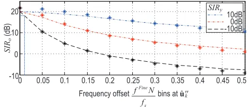
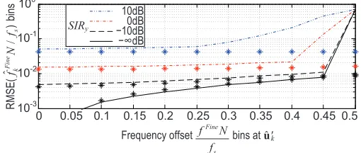
Fig. 5 shows how the output SIR is degraded with frequency offsets measured in bins (equivalent to an N-point FFT bin size of fbin = fs/N Hz). The discrepancy between the simulations and theoretical is caused by the error in the first term as previously explained and the loss of the low angle assumption at larger fF ine_{s. It is to be noted that} _SIR

o deteriorates with small frequency offsets, especially whenyk has a significant interference componentuk. Frequency offset should be less than 0.01 bins (i.e., fF ine < 0.01fs/N Hz),

if SIRy = −10dB, and the implementation loss is to be

restricted to less than 2dB (as shown by the blue dotted lines in Fig. 5). This is the goal of frequency correction discussed next.

B. Coarse Frequency Correction

The fine frequency correction module requires the residual frequency offset to be within±0.5bins, therefore a good target for the coarse frequency correction module is to reduce the residual frequency offsetfF ine_on_ˆ_u′

k to within 0.25 bins (i.e. fF ine_≤₀_.₂₅_f

s/N Hz). Hence, from (24) we have,

∆f−0.25fs/N≤fCoarse≤∆f+ 0.25fs/N. (51)

As discussed earlier in section III-C, the coarse correction module is accurate within 0.5 bins of the M-point FFT (equivalent to 0.5fs/M Hz). Hence, evaluating 0.25fs/N = 0.5fs/M gives the required number of FFT points on the coarse correction moduleM = 2N (8192).

However, the M-point FFT can be forced into error by the presence ofs iny. In the worst case scenario where the frequency offset is on a bin boundary, the target residual offset (fF ine≤0.25fs/N Hz) is achieved if the highest power bin lmax is one of the two bins on either side of the offset bin boundary. The solid line (blue) Fig. 6 shows the probability of lmax being one of the two bins for increasing powers ofs (i.e increasing SIRy). At SIRy = 10dB, the probability of fCoarse_{being within range (51) is 97%. But values of}_SIR

(8)

0 20 40 60 80 100

25 20

15 10

5 0

SIRy(dB)

FFT

Points M=8N

M=2N M=16N M=32N

P

ro

ba

bi

lit

y

(%

)

Fig. 6. Probability of acceptable coarse frequency correction (∆f−0.25fs/N≤fCoarse≤∆f+ 0.25fs/N) forM= 2N,M= 8N, M= 16NandM= 32N.

greater than 10dB force lmax outside the two expected bins and the probability falls exponentially.

The performance at higher SIRys can be improved by increasing the number of FFT points M. This reduces the FFT bin sizes and its susceptibility to noise. It also increases the number of frequency bins that result in acceptable coarse correction. For example, a M = 8N-point FFT results in 0.125fs/N Hz bin sizes andlmaxcould be any one of 4 bins (two on either side of the offset bin boundary). Fig. 6 further illustrates the probability of fCoarse _{being within range (51)} for M = 8N,M = 16N andM = 32N.

C. Fine Frequency Correction

The fine frequency correction module removes any re-maining offsets after the initial coarse correction stage. The module is designed to operate within offsets of±0.5 bins (i.e., fF ine _<_|₀_.₅_f

s/N| Hz). There are two factors that affect the accuracy of the estimate fˆF ine

k , a)

1) the level of desired signalsk inyk that acts as interfer-ence to the estimation process, and

2) the absolute value of frequency offsetfF ineon the input signalˆu′_k.

Expanding (32) by splitting y into its signal and distortion components and then using equation (22) and (29), gives,

ϕk= 1 N

N ∑

n=1

sn,kuˆ′∗n,k+ 1 N

N ∑

1

ρˆu∗_n,kuˆn,ke−j(ψk− θ

2+

θn N).

(52) The linear phase shift is caused by the residual frequency offset fF ine_{, and} _ψ

k is the mean phase offset of the block. The mean ϕ¯k ≈ρ σu2ˆe−

jψk _{comes from the second term, and is}

accurate when θ is small. The variance of the first term is σ2

ϕk,1 =σ

2

sσ2uˆ/Ns. This variance is circularly symmetric and so the contribution to the phase error is a half of this value. The variance of the phase due to the first term is therefore,

σ2_̸ _ϕ k,1 =

1 2

σ2 sσu2ˆ ρ2_σ4

ˆ uNs

= SIRy

2Ns

. (53)

After the angles have been subtracted (i.e., ∆̸ ϕ = ̸ ϕk− ̸ ϕk₋1 ), the fine frequency estimate fˆkF ine is obtained from (34). The variancefˆ_kF ine due to the first term in (52) becomes,

σ2_ˆ fF ine

k,1

= SIRy

4π2_N s

( fs N

)2

. (54)

10-3 10-2 10-1

100

0 0.05 0.1 0.15 0.2 0.25 0.3 0.35 0.4 0.45 0.5

SIRy

10dB

10dB0dB

!dB

u'k

s

f N

f

RM

S

E

(

__

_

)

bi

ns

ˆ

/

F

in

e

k

s

f

N

f

Fig. 7. Performance with feedforward fine frequency correction. ‘*’s represent theoretical results.

The second term of (52) contributes an additional variance when fF ine _̸_{= 0} _{resulting in a linear phase shift} _θ _over the block. This makes the phase of ϕk dependent on the amplitudes of the individual uˆ′_n,k samples. The variance of

ˆ

f_kF ine due to frequency offset is derived in the appendix B and the overall estimate fˆF ine

k becomes,

ˆ

f_kF ine =N

{

fF ine, SIRy 4π2_N

s (

fs N

)2 +

( fF ine)2

24Ns }

. (55)

Fig. 7 shows the root mean square error of fˆF ine k (i.e.,

RMSE( ˆf_kF ine) =

√

E{( ˆf_kF ine−fF ine₎2_}_{) as a function of} the actual frequency offset fF ine_{. The solid black line} rep-resents an input yk without any sk (i.e. yk = uk and SIRy = 0). The increase in RMSE( ˆfkF ine) with frequency offset is from the second term only. When SIRy ̸= 0 the minimum RMSE( ˆfF ine

k )level is set by the first term of (52). There is good agreement between simulations and theory for frequency offsets below 0.25 bins (i.e., fF ine < 0.25fs/N Hz). When the frequency offsetfF ine goes beyond 0.5 bins (0.5fs/N Hz) the phase difference ̸ ϕk −̸ ϕk−1 crosses π and the estimate fˆ_kF ine jumps from 0.5 bins to −0.5 bins, a catastrophic situation. In the diagram the variance in the phase

̸ ϕk causes fˆkF ine to jump prematurely at lower frequency offsets, indicated by the steep rise in RMSE. This scheme will only work if the residual frequency offsetfF ine _{after the} coarse correction is≪0.5bins (i.e.,fF ine _<<₀_.₅_f

s/NHz).

D. Improved Feedback Fine Frequency Correction

An improved architecture with a feedback fine frequency correction is proposed to reduce the probability of exceeding the discontinuity at fF ine _{= 0}_.₅ _{bins (0}_.₅_f

s/N Hz) as well as reduce the averaging error caused by frequency offsets in (55). We correct the frequency offset prior to estimating̸ ϕk, as shown in Fig. 8,

ˆ

u′′n,k= ˆu′n,ke−j2π ˆ

f_kF ine₋₁ n/fs_. ₍₅₆₎

The correlator C now only has to calculate the change infF ine between blocks. An integrator holds the total estimatefˆF ine

k ,

ˆ

f_kF ine= ˆf_kF ine₋₁ + ∆̸ ϕ fs/2πN. (57)

(9)

( )

*

!

1

z

1

z

+ -+ +

{}

E

{}

E

( )

-1

GPA

Fine Frequency

Correction Correlator C Gain Phase Correction

k

yk

k

u'' u'''k

+

-D

e

m

o

d

u

la

to

r

k

o

ˆFine k

f

1

ˆFine k

f"

ˆ_k

#

Integrator

k

u'

Fig. 8. Proposed feedback fine frequency correction.

bins (0.5fs/N Hz) can now be tracked. The key requirement is that the change in frequency per block must be ≪ 0.5 bins. Fig. 9 shows the improved performance with respect to fF ine_{, the contribution from the second term in (55) is} nearly eliminated. Fig. 10 compares the two schemes track-ing a frequency drift of magnitude 10−5 bins per sample (10−5fs2/N Hz/sec). The feedforward scheme fails to track the frequency offset once it drifts beyond 0.5 bins (in line with previous observations in Fig. 7). This is because the feedforward scheme calculates the total frequency offset ofuˆ′_k relative to uk in each block stage. In contrast, the feedback scheme continues to track without any failures, since it only estimates the extra frequency offset that the current block has after correcting it with fˆF ine

k−1 (which is the total tracked frequency offset at the previous block). However, the feedback design of the scheme makesfˆF ine

k to fall short of tracking the exact offset, because the offset keeps increasing with every sample; as demonstrated in the figure, the feedback scheme’s tracking runs below the ideal tracking line.

Finally, it is to be noted that the feedback scheme can only track frequency drifts when it starts with small frequency offsets less than 0.5 bins (0.5fs/N Hz) depending on SIRy. As observed earlier in Fig. 9, it can fail to track when starting with frequency offsets that are too high (e.g., 0.43 bins for

SIRy= 10dB).

V. PRACTICALMEASUREMENTS

In this section, a practical setup in accordance to Fig. 2 is used to demonstrate that two out-of-band jammers at

10-3

10-2 10-1 100

0 0.05 0.1 0.15 0.2 0.25 0.3 0.35 0.4 0.45 0.5

SIRy

10dB

-10dB0dB

u_'_k Frequency offset_______ Fine bins at

s

f N

f

R

M

S

E

(

__

_

)

bi

ns

ˆ

/

F

in

e

k

s

f

N

f

Fig. 9. Performance with feedback fine frequency correction.

-0.5 0 0.5 1 1.5 2

0 0.2 0.4 0.6 0.8 1 1.2 1.4 1.6 1.8 2

feedforward

feedback

ideal tracking

u_'_k

s f N

f

bins

ˆFine k

s f N

f

Fig. 10. Frequency drift tracking byfˆF ine

k .

a colocated setting generate reverse IM3 products causing major interference for the victim receiver. Further, a prac-tical implementation of our proposed receiver architecture is demonstrated using Universal Software Radio Peripherals (USRPs) [22] as SDR front-ends. The signals are data-logged and processed in MATLAB.

Fig. 11 shows the two jammer antennas (A and B) colocated at close proximity to one another. Each jammer is a signal generator, QPSK modulated with an USRP and amplified by a power amplifier (Mini-Circuits ZHL-42W [29]),

trans-Jammer Signal Generators

USRP for QPSK

40cm

Power Amplifiers Jammer A

@922MHz Jammer B@477MHz

(10)

Unit dBm SWT 5 ms

RBW 2 MHz VBW 2 MHz Ref Lvl

-15 dBm Ref Lvl -15 dBm

RF Att 10 dB

-110 -100 -90 -80 -70 -60 -50 -40 -30 -20

Span 1.5 GHz

Center 750 MHz 150 MHz/

IM3 Product

@1367MHz

Jammer A

@922MHz

Jammer B

@477MHz

IM2 Product

@1399MHz

3rd

Harmonic

@1431MHz

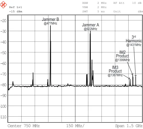
Fig. 12. Frequency spectrum of the jammers and distortions at RX’s antenna.

mitting with an omni-directional dipole antenna. A small separation of 40cm is required to generate a considerable reverse IM3 product at the low transmitting powers in the laboratory setting. Jammer A transmits a 0.5W signal at 922MHz and jammer B transmits a 1W signal at 477MHz, this propagates into the power amplifier of jammer A and produces a reverse IM3 product at 1367MHz. Fig. 12 shows the frequency spectrum at the victim receiver RX’s antenna. Adjacent to the 1367MHz reverse IM3, the spectrum shows the 1399MHz (922MHz+477MHz) reverse second-order in-termodulation (IM2) product and the 1431MHz (3x477MHz) third harmonic, these signals are at sufficient separation and do not affect our experiment.

Victim receiver RX is setup in accordance to our proposed receiver architecture using three crystal locked USRP units Rx0, Rx1 and Rx2 as seen in Fig. 3. The victim antenna is placed 3m from the out-of-band jammers A and B to ensure that they do not overload the receiver front-ends. To demonstrate the performance of the receiver system a narrow-band 12.5 kHz QPSK modulated signal is used for both the desired and jammer signals. The symbol rate is 7.8125 ksymbols/s and filtered with a Nyquist filter with 50% excess bandwidth. Fig. 13 shows the constellation of the desired signal and a 0.5MHz baseband spectrum received at Rx0.

Fig. 13(a) shows the reception of the desired signal at Rx0 without any jammers and interference. The receiver is operated at low IF to avoid any DC offset issues. The low-powered transmitter for the desired signal is mounted in an adjacent room. The scatter plot on the left hand side shows the four QPSK constellation points of the received desired signal at a signal-to-noise ratio (SNR) of about 38dB.

Fig. 13(b) shows the spectrum at Rx0 with the out-of-band colocated jammers turned on. The reverse IM3 product from jammer A falls directly on the desired signal frequency (1367MHz) and completely masks the signal causing major interference. The constellations have an SIR=2dB and are

unrecognizable as a result of interference.

Fig. 13(c) shows the spectrum after DSP correction. The inset compares the spectrum (black) of the DSP corrected signal with the spectrum (blue) of the IM3 distorted signal. Error vector magnitude measurements on the constellation diagrams indicate that the IM3 distortion has been canceled by 16dB, leaving the desired signal with a SIR of about 18dB. The DSP is implemented in MATLAB in accordance to our simulation settings with OSR = 64, N = 4096 and M = 2N. As in Fig. 3, the DSP takes inputs from Rx1 and Rx2, synthesizes a copy of the IM3 and removes it from the primary reception at Rx0. The18dB SIR achieved is in close agreement to the20dB output SIR achieved in our simulations (Fig. 4).

Fig. 14(a) and (b) show the baseband frequency spectrums on Rx1 and Rx2 respectively. Rx1 receives the 922MHz jammer A at a frequency offset of 55kHz and Rx2 receives

Constellation

A

mplit

ude

(

dB

)

Frequency (MHz) -1

-0.5 0 0.5 1

-1 -0.5 0 0.5 1

-40 -20 0 20 40

-0.1 0 0.1 0.2

-0.2

(a) Without interference from reverse IM3

Constellation

A

m

p

lit

u

d

e

(d

B

)

Frequency (MHz) -1

-0.5 0 0.5 1

-1 -0.5 0 0.5 1

-40 -20 0 20 40

-0.1 0 0.1 0.2

-0.2

(b) With interference

Constellation

A

m

p

lit

u

d

e

(d

B

)

Frequency (MHz)

-1 -0.5 0 0.5 1

-1 -0.5 0 0.5 1 -40 -20 0 20 40

-0.1 0 0.1 0.2 -0.2

-20 0 20-10 0 10 20

(kHz)

(c) With interference and cancellation system

(11)

A

m

p

lit

u

d

e

(d

B

)

Frequency (MHz)

-40 -20 0 20 40

-0.1 0 0.1 0.2 -0.2

A

m

p

lit

u

d

e

(d

B

)

Frequency (MHz)

-40 -20 0 20 40

-0.1 0 0.1 0.2 -0.2

(a) Spectrum at RxA (b) Spectrum at RxB

Fig. 14. Frequency spectrum of the jammers.

the477MHz jammer B at a frequency offset−45kHz. The RF gain on the front-ends are attenuated such that the jammers are within the receiver’s dynamic range. Appendix C shows the auxiliary receiver’s dynamic range requirements are modest and related to the amount of cancellation required. It should be noted that the jamming signals are significantly larger than the reverse IM3 product (approx. 40-50dB as seen in Fig. 12). If receiver distortion occurs, there is plenty of scope for attenuating the jammers without affecting the quality of the synthesized IM3 estimateuˆ.

Fig. 15 showsfˆF ine

k ’s fine frequency tracking of the aggre-gated local oscillator drifts. As estimated, the coarse frequency correction module has reduced the frequency offset to about 0.25 bins (0.25fs/N Hz). The ripples seen in the figure are primarily due to RMSE( ˆfF ine

k ) caused by the interference effect of the desired signal in the fine frequency estimation algorithm.

We now consider practical aspects of fielding such a so-lution. The implementation penalty is dominated by the cost and power consumption associated with the additional receiver chains and their ADCs. Multiple receiver chains on a single integrated circuit are becoming available because of diversity and MIMO requirements in the new standards. The cost and energy consumption continues to drop. An approximate power budget would allow 0.2W per receiver chain [30]. The traditional transmit side solution of filters and isolators involve bulky high power components with insertion loss and often poor frequency agility. A 20W transmitter with two isolators has an additional 1dB insertion loss [31], which represents a dissipation loss of 5W, clearly more than the receiver side solution proposed here.

0 0.1 0.2 0.3 0.4 0.5

k-th block

0 20 40 60 80 100 120 140 160 180 200

12.2Hz

1.64s

bins ˆFine

k

s

f N

f

Fig. 15. Fine frequency tracking byfˆF ine

k .fs=0.5Msamples/s,N=4096.

VI. CONCLUSION

Reverse IM products, signal harmonics and other distortions may fall on the desired receive channel of a colocated receiver and cause interference. The paper describes a postdistortion cancellation system for the victim receiver. A distortion regen-eration circuit is used to synthesize an estimate of the reverse IM from the jamming signals. This is then used to mitigate (cancel) the distortion on the desired signal. The scheme is flexible and can be used to cancel not only a single reverse IM product but also multiple distortion products, jammer harmonics and any form of distortion where the constituent jamming signals are available. This includes IM products generated within the desired receiver itself. Each different product requires its own generating function and frequency offset correction. The subtraction is done sequentially with the strongest distortion component subtracted first (Fig. 1). The scheme does not need to know the desired signal, s, whose amplitude and phase remains unaffected by the algorithm. As such, signal processing algorithms associated with multiple an-tenna receivers will not be affected by the canceling. Note, the non-linear polynomial function and frequency offset correction can be a common circuit, but separate gain-phase corrections are required for each receiver chain.

A multi-front-end receiver architecture was used to ensure tracking of out-of-band jammers without the need for ex-tremely high sampling frequencies. This can lead to frequency offsets between the estimate and the reverse IM3 product. The proposed scheme uses a two stage frequency offset correction technique, an FFT for coarse correction and signal correlation for fine frequency tracking. A differential feedback tracking scheme was also devised to track frequency drifts beyond the coarse correction capability. The scheme uses Bussgang’s minimum mean squared error formula to correct the estimate’s amplitude and phase.

Mathematical analysis and simulations were used to com-prehensively characterize the system. The results were then validated in hardware. It was shown that the desired signal acts as noise to the correlator outputs controlling the frequency off-set correction and gain phase correction coefficient. To counter this, averaging and increased FFT sizes were necessary.

The output SIR (SIRo) was shown to be dependent on the equivalent number of uncorrelated samples (Ns) in the aver-aging block. The maximum SIR improvement possible was shown to be (Ns−SIRy)dB. Therefore, it is recommended to switch OFF the canceling circuit whenSIRy< Ns.

The paper demonstrated a working prototype of the postdis-tortion cancellation system. Jammers at frequencies 477MHz and 922MHz caused a reverse IM3 product at 1367MHz which is within the GPS3 satellite band. The cancellation algorithm achieved an 18dB output SIR that is in close agreement with the simulation and analytical results. The input SIR was 2dB indicating a 16dB reduction in the reverse IM3 distortion. Had the input SIR been worse, the cancellation would have been correspondingly higher. Table I summarizes related work in distortion cancellation.

3_{GPS signals are very low level and are particularly sensitive to noise and}

(12)

2

N

1 N

4 2

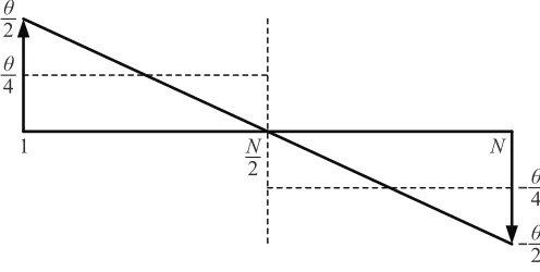
2 4

Fig. 16. Linear phaseθ(= 2πfF ine_N/f

s) across a block.

APPENDIXA

THEMODULATIONPARAMETERFACTORη

The variance of the signal ϕ′_k from the correlation of ˆu′′_k with sk (the desired signal component in yk) is obtained by calculating the power spectrum P(f) of the signal (skˆu′′k) and then multiplying it with the power frequency response of the averaging function. AnN-point averaging filter has a low pass frequency response, with an effective power bandwidth of fs/N (where fs is the sampling frequency). We make an approximate solution for the case where all signals have the same bandwidth of fs/OSR and a rectangular spectral shape. If the desired signalsk with spectrumS(f)was passed through the averaging filter, its variance would be reduced by ηN/OSR, whereη= 1.

The spectrum P(f) is a convolution of S(f) with the spectrum Uˆ(f) (of the IM3 distortion signal ˆu′′_k), which itself is a triple convolution of the spectrums A(f), A(f) and B(f) (of the fundamental jammer signals a andb). i.e. P(f) =S(f)∗Uˆ(f) =S(f)∗A(f)∗A(f)∗B(f). There are 4 convolved terms. We note that the convolution of two unit rectangular signals (power spectral density=1, bandwidth=1) is triangular in shape (magnitude=1, bandwidth=2), and the convolution of two triangles give a signal with a magnitude spectrum of 2/3 at the center of the band (at DC). Since N is large, the averaging filter bandwidth is very small and we assume a constant spectrum of P(0) over its bandwidth. The variance is, therefore, reduced by (9/4)N/OSR, giving η = 9/4. Of course, the magnitude of A(f) and B(f) also has an effect on the variance, but this is accounted for by the normalization whenϕ′_k goes toρˆk.

APPENDIXB

THEVARIANCE OFfˆ_kF ine DUE TOFREQUENCYOFFSET

The linear phase shift of θ across the block in the second term in (52) produces an orthogonal errorϵk inϕk, the mean of which is zero. For small θ,

¯ ϵk=

1 N

N ∑

1

ρuˆn,kuˆ∗n,k (

θ

2 −

θn N

)

e−jψk _{= 0}_. ₍₅₈₎

We now split the summation into 2 parts (Fig. 16). The mean for the first and secondN/2samples is¯ϵk,1=

(_θ

4

) ρσ2

ˆ ue−jψk and¯ϵk,2=

(

−θ 4

) ρσ2

ˆ ue−

jψk_{respectively. The variance for both}

halves are,

σ_ϵ2_k,₁ =σ_ϵ2_k,₂= _N2 N/_∑2

1

ρ2σ4_u_ˆ{(θ₂−θn_N)−(θ₄)}2

=θ2

48ρ

2_σ4

ˆ u.

(59)

When we average over allN samples the mean goes to zero and the variance becomesσ2

ϵk= θ2

48Nsρ

2_σ4

ˆ

u. We then substitute for θ as per (46), and change back to a phase error σ2

̸ ϕk =

tan−1(_σ2 ϵk/

¯ ϕk

2)

by using the small angle approximation. The phase error variance is doubled after the subtraction of (33) to give fˆ_kF ine. Thus, the variance of fˆ_kF ine due to the second term in (52) becomes

σ_f2ˆF ine k,2

=

( fF ine)2

24Ns

. (60)

APPENDIXC

AUXILIARYRECEIVERDYNAMICRANGE

We show that the maximum level of IM cancellation deter-mines the minimum dynamic range of the auxiliary receivers. If the auxiliary receivers include noise (and other error) terms, na and nb, from receiver Rx1 and Rx2 respectively, then equation (19) becomes:

ˆ

u=b∗a2+ 2b∗a na+a2n∗b+O(n2) (61)

where the sub-scripts have been dropped for clearer under-standing. The first term is the wanted regenerated distortion term and the second and third terms are the most dominant error terms. The others are much smaller and neglected. Even if there is perfect cancellation of the distortion term in equation (37), these error terms remain and corrupt the desired signal, forming a floor toSIRo. The maximum cancellationCmax is therefore given by,

Cmax(=SIRo/SIRy) =E{|b∗a2|2}/E{|2b∗a na+a2n∗b|

2_}

(62) For example, if we assume b ∼ a, na ∼ nb, then Cmax = E{|a|2_}_/₅_E_{|_n

a|2} or Cmax(dB)= −7(dB)+SNRa(dB). A 30dB maximum cancellation limit would call for auxiliary receiver dynamic ranges of 37dB, leading to ADC resolutions of at least 7 bits provided quantization noise was the dominant error source.

REFERENCES

[1] K. Allsebrook and C. Ribble, “VHF cosite interference challenges and solutions for the United States Marine Corps’ expeditionary fighting vehicle program,” inProc. IEEE Military Communications Conference, 2004.

[2] F. German , K. Annamalai, M. Young , M. C. Miller, “Simulation and Data Management for Cosite Interference Prediction,” inProc. IEEE International Symposium on Electromagnetic Compatibility, July 2010. [3] I. Demirkiran, D. D. Weiner, A. Drozd and I. Kasperovich, “Knowledge-based Approach to Interference Mitigation for EMC of Transceivers on Unmanned Aircraft,” in Proc. IEEE International Symposium on Electromagnetic Compatibility, July 2010.