A New Adaptive Tracking Algorithm for Near-Space
Hypersonic Target
Xiangke Guo1, *, Changyun Liu2, Qiang Fu2, and Gang Wang2
Abstract—Because of the maneuvering of hypersonic target, the tracking of near space hypersonic targets is difficult. In this paper, a new adaptive tracking algorithm based on an aerodynamic model and improved square root cubature Kalman filter is proposed. The adaptive piecewise constant jerk model gives the acceleration recursive process based on the dynamic model. Considering the nonlinear characteristic of both the target state model and the observation model, the improved square-root cubature Kalman filter is applied to estimate the target state. The simulation results under different maneuvers conditions indicate that the proposed method has a higher degree of accuracy than the original aerodynamic model. The research provides a feasible solution to the further improvement of the real time tracking accuracy of near space hypersonic targets.
1. INTRODUCTION
As projects related to near space hypersonic targets (NSHT) [1–3] developed by the U.S. forces gradually mature, NSHT with characteristics of expansive flight cross-domain, high velocity and complex aerodynamic parameter variation pose a challenge to the intercept and attack abilities of air defense and anti-missile systems [4–6]. Many studies have been conducted that deal with the motion modeling and tracking algorithm of NSHT. At present, the dynamic model based on a gravity turning frame and aerodynamic pressure is widely used for space targets and ballistic targets [7]. Wu and Chen used the aerodynamic model to estimate the motion state along with aerodynamic parameters [8]. However, the model has complex interactions and requires a large computational load. According to the dynamic characteristics of the air-breathing hypersonic target Li et al. proposed the dynamic hybrid model set for target tracking [9]. However, the analytical solution structure is difficult to implement for a linear filter design. To address the shortcomings of the traditional dynamic, Zhai et al. proposed a new aerodynamic model to realize the trajectory prediction of a hypersonic target. However, since no aerodynamic acceleration recursive step is given, the model cannot be directly used for filtering [10, 11]. Therefore, on the basis of the aerodynamic model in papers [10] and [11], a piecewise adaptive jerk tracking model of NSHT is proposed. The square root cubature Kalman filter (SRCKF) is used to accomplish the filter tracking of a target. This filter has better nonlinear approximation features, numerical accuracy, small computation and suitability for real-time calculation [12–14]. Finally, the effectiveness of the new adaptive tracking algorithm is verified by simulation.
2. THE DYNAMIC MODEL OF NSHT
The acceleration model of a maneuvering reentry target can be written as [7]:
d2r
dt2 =a+g−ωe×(ωe×r)−2ωe×v (1) Received 1 July 2018, Accepted 4 September 2018, Scheduled 19 September 2018
* Corresponding author: Xiangke Guo ([email protected]).
wherer,v,g,ωeandaindicate the earth vector of a target, flight speed of a target, gravity acceleration,
earth rotation angular speed and aerodynamic acceleration. Also, −ωe×(ωe×r) indicates inertial centripetal acceleration, and−2ωe×v indicates Coriolis acceleration.
The aerodynamic acceleration a is the main factor affecting the maneuver of the target, and its change determines the maneuvering state of the aircraft. Therefore, the inertial centripetal acceleration and Coriolis acceleration in the total target acceleration can be ignored. The gravity accelerationg can be respectively modeled as a flat model, ball model and ellipsoid model. Here, focus on the modeling of aerodynamic accelerationa.
3. PIECEWISE-CONSTANT JERK MODEL
3.1. The Piecewise-Constant Acceleration Model
According to the concept of piecewise uniform acceleration (Piecewise-Constant Acceleration, or PCA) [7], under an ENU coordinate system, using aerodynamics parameterαVTC model aerodynamics
acceleration can be stated as [10]:
¨
x=αVP0x˙−αTP0v
˙
y vg −
αCP0
˙
xz˙
vg
¨
y=αVP0y˙+αTP0v
˙
x vg
αt−αCP0
˙
yz˙
vg
¨
z=−αVP0z˙+αCP0vg−g
(2)
where ¨xk, ¨yk, ¨zk are the acceleration components along the three axes in the ENU system; P0 is the
free flow of pressure; vis the target speed; αV T C = [αV, αT, αC]T is the aerodynamics parameter. The
relationship between the aerodynamic parameterαV T C and the acceleration of the target in the VTC
coordinate system isaV T C = [aV;aT;aC ] = [αVP0v;αTP0v;αCP0v].
From Eq. (2), it can be seen that the PCA model does not give a recursive equation for aerodynamic acceleration. In each filtering cycle, the target acceleration cannot be directly corrected using innovation. Therefore, if either the target maneuver or the initial state setting is inaccurate, the likelihood of a system tracking error will increase. When a recursive model of acceleration is established in the state equation, the state model can rectify the acceleration item recursively, according to the observational innovation of the sensor in each filtering period. That can improve the estimation accuracy of the system state. Therefore, in this paper, based on the previous aerodynamic model, the recursive equation of the target aerodynamic acceleration is established, and a piecewise constant Jerk adaptive tracking model for tracking hypersonic targets is proposed.
3.2. The Piecewise-Constant Jerk Model
Suppose that the jerk value of the NSHT is uniform in the sampling interval. According to random model approximate thought [15], taking random error into the acceleration recursion equation, the acceleration recursion equation is defined by:
[ x¨ k+1
¨
yk+1
¨
zk+1 ]
=
[ x¨ k
¨
yk
¨
zk ]
+
[ ...
xk
...
yk
...
zk ]
T+wk (3)
wherewk is defined as the acceleration vector at timekand the error which is generated by the random
error of jerk acceleration at time k+ 1,wk= [
˜ ¨
xk+ ˜
...
xkT y˜¨k+ ˜
...
ykT z˜¨k+ ˜...zkT ]T.
From Eq. (3), the subsection uniform jerk model state equation under an ENU coordinate system is generated by
Xk+1 =FCAXk+GJJ(Xk,pk) +WCJk (4)
where Xk = (xk,x˙k,x¨k, yk,y˙k,y¨k, zk,z˙k,z¨k)T is the target state vector; FCA = blkdiag(F, F, F) is the
state transition matrix; GJ = blkdiag(Gx,Gy,Gz) is the jerk input matrix, and Gx = Gy = Gz =
[
J(Xk,pk) = [
...
xk
...
yk ...zk ]T is the jerk of the target; WCJk is the Gaussian noise of covariance
matrix QCJk ; QCJk = blkdiag(σ2axqCA, σ2ayqCA, σ2azqCA), σax2 , σay2 and σaz2 are instantaneous variances of acceleration in thex,y and z directions, respectively. Also, F and qCA are defined as:
F =
1 T
T2
2
0 1 T
0 0 1
, qCA =
[ 0 0 0
0 0 0 0 0 qaT
]
Where qa is the steady state precision adjust factor, according to Eq. (2), and J(Xk,pk) is computed
by ...
x =αVP0x¨−αTP0 (
˙
vy˙ vg
+v y¨ vg −
v y˙ v2
g
˙
vg )
−αCP0 (x¨z˙
vg
+x˙z¨
vg −
˙
xz˙
v2 g ˙ vg ) ...
y =αVP0y¨+αTP0 (
˙
vx˙ vg
+v x¨ vg −
vx˙ v2 g
˙
vg )
−αCP0 (y¨z˙
vg
+ y˙z¨
vg −
˙
yz˙
v2 g ˙ vg ) ...
z =αVP0z¨+αCP0v˙g
(5)
wherev=√x˙2+ ˙y2+ ˙z2 is the flight speed of the target, v g=
√
˙
x2+ ˙y2, ˙v= x¨˙x+ ˙yy+ ˙¨ z¨z v , ˙vg =
˙ x¨x+ ˙yy¨
vg .
Supposeσak2 =[ σax2 σay2 σaz2 ]T, the instantaneous variance of acceleration is generated by
σ2ak = diag
(
[˜¨xk˜¨x T
k] +T2[˜
...
xk˜
...
xTk] + 2T[˜¨xk˜
...
xTk]
)
(6)
where ˜¨xk= [ ˜
¨
xk y˜¨k z˜¨k ]T
is the acceleration estimation vector, and ...x˜k = [
˜ ...
xk ˜
...
yk ...˜zk ]T is the jerk estimation error vector. When ignoring the product of the jerk and acceleration error, the variance expectation of acceleration and jerk are similar to the instantaneous variance. Therefore, Eq. (6) can be defined by
σ2ak = diag
(
CaE[˜¨xk˜¨x T
k] +T2CJE[˜
...
xk˜
...
xTk]
)
(7)
where Ca and CJ, respectively, are the acceleration and jerk variance conversion coefficient. The
recursion of aerodynamic parameters in the segmented uniform jerk model can be achieved by separately calculating E[xk˜¨ ˜¨xTk] and E[...˜xk˜
...
xTk], using different filtering algorithms.
4. IMPROVED SQUARE ROOT CUBATURE KALMAN FILTER
4.1. Square Root Cubature Kalman Filter
Considering the nonlinear characteristics of the target state model and the observation model, the nonlinear approximation performance and numerical accuracy are better than those of other nonlinear filtering algorithms. The algorithm has a small computational load and is more suitable for real-time calculation. The cubature Kalman filter (CKF) has higher filtering precision than the Unscented Kalman filter (UKF) when the dimensionality of the target state is greater than 3. In the process of CKF, the error covariance matrices need to be decomposed and inverted. However, it is difficult to guarantee the positive definite of the error covariance matrix. Therefore, the state-filtering of the target is avoided by introducing Cholesky decomposition, in order to avoid the square root cubature Kalman filter (SRCKF), which directly performs the square root operation on the covariance matrix and has better filtering stability [12–14]. The SRCKF avoids the square root operation of the iterative matrix by introducing orthogonally triangular decomposition. However, the SRCKF directly calculates the square root of the covariance matrix. It solves the easy divergence issue of a conventional CKF algorithm and improves the accuracy and stability of filtering.
To realize the recursive estimation of the hypersonic target aerodynamic parameterpin the adjacent space, the segment jerk model is extended as a state estimation parameter, and the extended jerk motion model is shown in Eq. (8), as follows:
[ Xk+1 pk+1 ] = [ FJ 0 0 I ] [ Xk pk ] + [ GJ 0 ] Jk+
[ WJk Wpk
]
whereWpk is the parameter of Wiener model process noise, andQpk is the covariance matrix. Combine
Eq. (8) with the measure equation, and the result is as follows:
{
Xak=f(Xka−1) +Wak−1 Zk =h(Xak) +Vk
(9)
where Xak−1 = (XTk−1,pTk−1)T; Wka−1 = [(WkJ−1)T,Wp,kT −1]T, h(Xak) is a nonlinear function between the measured value and the state value, and the measurement noise Vk is a zero-mean Gaussian white
noise vector with variance Rk.
Suppose the posterior probability distribution of the known state estimation is p(xak−1|z1:k−1) ∼
N(xak−1;ˆxak−1, Pka−1), the corresponding covariance is Pka−1, and the expanded model progress noise covariance matrix is Qak = blkdiag(QJk,Qpk); then Sax,k = chol(Pak) is a Cholesky decomposition. The
SRCKF algorithm based on the expanded status model is defined as follows: (1) Calculate the basic cubature points and the corresponding weights.
The nonlinear filtering problem under Gaussian distribution can be reduced to an integral calculus problem. The standard Gaussian weighted integral can be calculated by using the third-degree spherical radial rule and 2nx volume points are needed. The basic cubature point and the corresponding weight
is:
ξi = √
m
2 [1]i, wi= 1
m, i= 1,2, . . . , m (10)
where the cubature point number is m,m = 2nx, andnx is the dimension of state; [1]i represents the i-th column of the complete symmetric point set [1].
(2) Time updates
Calculate the mcubature points of the current state (i= 1,2, . . . m),m= 2n.
Xi,ka −1|k−1=Sak−1|k−1ξi+ ˆxak−1|k−1 (11)
Calculate the predicted value of the volume point through the nonlinear state transfer function.
Xi,ka(∗|k)−1=f(Xi,ka −1|k−1) (12)
Estimate the predicted state (SRCKF uses equal weights) in conjunction with the weights and volume point predictions.
ˆ
xak|k−1 = 1
m m ∑
i=1 Xa(∗)
i,k|k−1 (13)
The square root of the estimated covariance matrix:
Sak|k−1 = Tria([χi,k|k SQ,k−1]) (14)
whereQa
k−1 =SQ,k−1SQ,kT −1, and
χi,k|k=
1
√ m
[ Xa(∗)
1,k|k−1 −xˆ
a k|k−1, X
a(∗)
2,k|k−1−xˆ
a
k|k−1, . . . , X a(∗)
m,k|k−1−xˆ
a k|k−1
] .
The algorithmS = Tria(A) means that matrixAis first QR-decomposed, and a normal orthogonal matrixB and an upper triangular matrixC are obtained. LetS =CT, and the resultingS is an upper triangular matrix.
(3) Measurement update (k= 1,2, . . .)
Calculate the updated state cubature points (i= 1,2, . . . , m).
Xi,ka |k−1=Sak|k−1ξi+ ˆxak|k−1 (15)
Calculate the predicted measurement cubature points.
Zi,k|k−1 =h (
Xa
i,k|k−1
)
Estimate predictive measurements.
ˆ
zk|k−1 = 1
m m ∑
i=1
Zi,k|k−1 (17)
The estimate of the innovation covariance matrix is:
Szz,k|k−1 = Tria([Zk|k−1 SR,k]) (18)
whereRk =SR,kSR,kT ,Zk|k−1 = √1m[Z1,k|k−1−zˆk|k−1, Z2,k|k−1−zˆk|k−1, . . . , Zm,k|k−1−zˆk|k−1]. Estimate
the cross-covariance matrix:
Pxz,k|k−1 =χk|k−1ZkT|k−1 (19)
Whereχk|k−1= √1m[X1,k|k−1−xˆk|k−1, X2,k|k−1−xˆk|k−1, . . . , Xm,k|k−1−xˆk|k−1].
Estimate the SRCKF filter gain.
Wak=
(
Pxz,k|k−1 /
Szz,kT |k−1 )/
Szz,k|k−1 (20)
Based on the new measurementzk at timek, the system state is updated.
ˆ
xak|k = ˆxak|k−1+Wk (
zk−zˆk|k−1 )
(21)
The square root factor of the error covariance matrix is updated.
Sk|k= Tria([χk|k−1−WkZk|k−1 WkSR,k]) (22)
(4) Calculation of instantaneous variance of acceleration
To achieve the recursion of the aerodynamic parameters in the homogeneous jerk model, the instantaneous variance of acceleration needs to be calculated. The diag(E[˜¨xk˜¨x
T
k]) in Eq. (8) can be
obtained directly from the state covariance matrices associated with the output of the k-time filter. That is, diag(E[˜¨xk˜¨xTk]);E[...˜xk˜
...
xTk] is calculated as follows: ...
x =J(x,x, y,˙ y, z,˙ z,˙ p) (23)
where ...x = [ ...x ...y ...z ]T is jerk vector. Construct the variable xn= [x,x, y,˙ y, z,˙ z,˙ p]T and the state covariance matrixPn. Then,
...
x =J(xn).
The state estimation valuexˆnand covariancePnare known at timek, and theE[˜
...
xk˜
...
xTk] calculation method based on the SRCKF is given by:
E[...˜xk˜
...
xTk] =E[(J(ˆxn+Sn,iξi)−J(ˆxn))(J(ˆxn+Sn,iξi)−J(ˆxn))T] (24)
where Sn = chol(Pn) is Cholesky decomposition Pn; Sn,i is the i-th line of Sn; nx is the dimension
number of xn; ξi is the number i basic cubature point. The covariance of the jerk estimation error
vector at timek can be calculated based on Eqs. (10), (13), (15), (18), and (19).
4.2. Model State Error Adaptive Estimation
When the tracking model is more accurate, the state covariance can reflect the state estimation error more accurately. When the model is mismatched, it will cause the tracking of the hypersonic target in the near space. Therefore, the state estimation of the target will worsen, or even diverge, resulting in a deterioration of target tracking performance. Therefore, in piecewise-constant ierk model, the state error coefficient of the tracking target is estimated by using the model mismatch detection functionDk
in real time. Also, the state error coefficient is transformed into the variance transformation coefficients
Ca andCJ to drive the change of state covariance.
The model mismatch detection function is:
Dk =vTkSzz−1vk (25)
where vk is innovation, and Szz is the innovation covariance of the filter output. As the position
the process of updating, the actual change of the jerk error covariance is more intense than that of the position and velocity error covariance when the target is maneuvering. Therefore, Ca and CJ are
defined by:
Ca= {
qaDk Dk>3 qa Dk≤3
, CJ = {
qJDk2 Dk>3 qJ Dk≤3
(26)
where qa and qJ are the designed parameters, which can be obtained from simulation. Therefore,
considering the model mismatch caused by target maneuver, the acceleration variance calculation method of Eq. (9) is modified as:
σak2 =
diag
(
qaDkE[x˜¨k˜¨x T
k] +T2qJD2kE[˜
...
xk...x˜Tk]
)
Dk>3
diag
(
qaE[˜¨xk˜¨x T
k] +T2qJE[˜
...
xk˜
...
xTk]
)
Dk≤3
(27)
After the above derivation and correction, the state covariance, covariance of the process noise and model mismatch detection function are correlated. When the target aerodynamic parameter estimation is accurate, the covariance of the process noise will decrease due to filter characteristics. The state covariance is reduced, and the state estimation error caused by the measurement noise is also reduced. The value of the model mismatch detection function increases, thus leading to an increase of covariance of the process noise when the target aerodynamic parameter changes cause the model mismatch. Also, the increase of covariance of the process noise will increase the state covariance. Mutual stimulation between the state covariance and the covariance of the process noise will greatly increase the gain of the algorithm filter, which in turn reduces the state estimation error.
5. SIMULATION RESULTS AND ANALYSIS
5.1. The Simulation Scene
A boost-glide hypersonic vehicle has significant differences with the phase of aerodynamics and ballistic target. This paper takes a boost-glide hypersonic vehicle as the simulation analysis object, in order to verify the effectiveness of the proposed algorithm in this paper. References [10] and [11] set the target simulation initial state as s1 = [0 km 0 km 40 km 2.4 km/s 0 km/s 0 km/s]T, and the radar
deployment position [500000 m 0 m 0 m]T. We set the radar standard deviation of range and angle measuring noise to 30 m and 0.05◦, respectively, and the sample interval is T = 0.1 s. The tracking algorithm process noise variance of acceleration is set to σax,k2 =σ2ay,k =σ2az,k = 52. In order to fully verify the effectiveness of the proposed algorithm, three typical motion modes of hypersonic targets are designed:
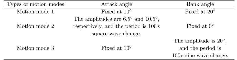
Table 1. The simulation parameters of three motion modes.
Types of motion modes Attack angle Bank angle
Motion mode 1 Fixed at 10◦ Fixed at 20◦
Motion mode 2
The amplitudes are 6.5◦ and 10.5◦, respectively, and the period is 100 s
square wave change.
Fixed at 0◦
Motion mode 3 Fixed at 10◦
The amplitude is 20◦, and the period is 100 s sine wave change.
5.2. The Simulation Results
0 2
4 x 10⁵ -10
-5 0
x 104 3 3.5 4
x 104
x/m y/m
z
/m
50 100 150 200 250 0
100 200 300 400 500 600
t/s
RM
S
o
f
p
o
si
ti
o
n
/m
PCA AIMM APCJ
50 100 150 200 250 0
20 40 60 80 100 120 140
t/s
RM
S
o
f
v
el
o
ci
ty
/
m
/s
PCA AIMM APCJ
50 100 150 200 250
0 5 10 15 20
t/s
RM
S
o
f
ac
ce
le
ra
ti
o
n
/
m
/s
2 PCA
AIMM APCJ
(b) (a)
(d) (c)
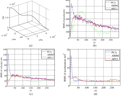
Figure 1. RMS of estimation error in Maneuvering Mode 1 conditions. (a) Motion path. (b) RMS of position error. (c) RMS of velocity error. (d) RMS of acceleration error.
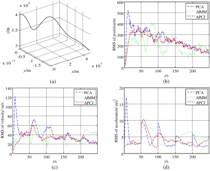
the adaptive interactive multiple model using 10 model sets (abbreviated as AIMM in the latter part of the simulation) in paper [11] and modified piecewise constant jerk (abbreviated as APCJ in the later simulation), as proposed in this article, combined with an improved SRCKF algorithm were simulated for the previous simulation scenario. In three different maneuvering conditions, the APCJ algorithm, AIMM algorithm and PCA algorithm were used in 50 Monte Carlo simulations. The position, velocity and acceleration root mean square (RMS) errors of the three algorithms are shown in Fig. 1, Fig. 2 and Fig. 3. In the three maneuvering conditions, the tracking performance statistics and calculation time statistics of the three algorithms are shown in Table 1, Table 2 and Table 3, respectively.
From Fig. 1, Fig. 2, Fig. 3, Table 1, Table 2 and Table 3, it can be seen that in the three different cases of maneuvering modes, the adaptive tracking method based on the piecewise constant jerk model (APCJ), adaptive interactive multiple model (AIMM) and piecewise constant acceleration model (PCA)
Table 2. Comparison of algorithm performance in Maneuvering Mode 1.
Types of algorithm
State Estimation Mean Error in Observation Time calculating time [s] Position/[m] Velocity/[m·s−1] Acceleration/[m·s−2]
APCJ 182.04 26.50 2.01 1.56
AIMM 184.09 25.58 2.25 3.89
0 2
4
x 105 -1.5
-1 -0.5 0
x 10-11 3 3.5 4
x 104
x/m
y/m
z
/m
50 100 150 200
0 100 200 300 400 500 600
t/s
RM
S
o
f
p
o
si
ti
o
n
/m
PCA AIMM APCJ
50 100 150 200
0 20 40 60 80 100 120 140
t/s
RM
S
o
f
v
el
o
ci
ty
/
m
/s
PCA AIMM APCJ
50 100 150 200
0 5 10 15 20
t/s
RM
S
o
f
ac
ce
le
ra
ti
o
n
/
m
/s
2
PCA AIMM APCJ
(b) (a)
(d) (c)
Figure 2. RMS of estimation error in Maneuvering Mode 2 conditions. (a) Motion path. (b) RMS of position error. (c) RMS of velocity error. (d) RMS of acceleration error.
Table 3. Comparison of algorithm performance in Maneuvering Mode 2.
Types of algorithm
State Estimation Mean Error in Observation Time Calculating time [s] Position/[m] Velocity/[m·s−1] Acceleration/[m·s−2]
APCJ 214.73 29.94 3.92 2.01
AIMM 213.62 35.36 4.01 3.79
PCA 232.94 38.35 4.02 2.29
Table 4. Comparison of algorithm performance in Maneuvering Mode 3.
Types of algorithm
State Estimation Mean Error in Observation Time Calculating time [s] Position/[m] Velocity/[m·s−1] Acceleration/[m·s−2]
APCJ 207.18 28.31 3.32 1.75
AIMM 219.83 31.96 3.88 3.91
0 2
4
x 105 -15000
-10000-5000 0 3
3.5 4
x 104
y/m
x/m
z
/m
50 100 150 200 250 300 0
100 200 300 400 500
t/s
RM
S
o
f
p
o
si
ti
o
n
/m
PCA AIMM APCJ
50 100 150 200 250 300 0
20 40 60 80 100 120
t/s
RM
S
o
f
v
el
o
ci
ty
/
m
/s
PCA AIMM APCJ
50 100 150 200 250 300
0 5 10 15 20
t/s
RM
S
o
f
ac
ce
le
ra
ti
o
n
/
m
/s
2 PCA
AIMM APCJ (b)
(a)
(d) (c)
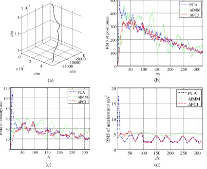
Figure 3. RMS of estimation error in Maneuvering Mode 3 conditions. (a) Motion path. (b) RMS of position error. (c) RMS of velocity error. (d) RMS of acceleration error.
based on the segmented uniform jerk model proposed in this paper is effective. It should be noted that, although the simulation results show that the tracking effect of the APCJ algorithm is better than that of the AIMM algorithm selected in this paper, this does not mean that the proposed algorithm is better than the AIMM. The degree of the tracking accuracy of the AIMM is closely related to the selection of sub-models, the number of sub-models and the parameter settings. The comparison between the proposed algorithm and the AIMM algorithm only shows that the proposed algorithm has tracking accuracy that is similar in degree to the AIMM, which greatly reduces the degree of computational complexity.
6. CONCLUSION
In this paper, the dynamic model of a near pace hypersonic target (NSHT) is modeled, based on the analysis of the aerodynamic characteristics of NSHT. Thus, the piecewise adaptive jerk tracking model is established, in order to accomplish the track of the NSHT with the improved square root cubature Kalman algorithm. The simulation results show that near space target tracking can be finished more effectively. Also, the proposed method is more precise in hypersonic tracking in near space than the segmental uniform acceleration model and the AIMM. Moreover, the proposed method increases the convergence performance and stability of the state tracking, especially when the target has lateral maneuvers. This algorithm is also effective in different simulation scenarios.
ACKNOWLEDGMENT
This paper is supported by the National Natural Science Fundation of China (No. 61503408).
REFERENCES
1. Huang, W., S. B. Luo, and Z. G. Wang, “Key techniques and prospect of near-space hypersonic vehicle,”Journal of Astronautics, Vol. 31, No. 5, 1259–1265, 2010.
2. Li, S. Y., L. X. Ren, Q. G. Song, et al., “Overview of anti-hypersonic weapon in near space,”
Modern Radar, Vol. 36, No. 6, 13–18, 2014.
3. Nie, W. S., S. B. Luo, and S. J. Feng, “Analysis of key technologies and development trend of near space vehicle,”Journal of National University of Defense Technology, Vol. 34, No. 2, 107–113, 2012.
4. Hu, Z. D., Y. Cao, and S. F. Zhang, “Trajectory performance analysis and optimization design for hypersonic skip vehicle,”Journal of Astronautics, Vol. 29, No. 3, 821–825, 2008.
5. Wang, L. D., Y. H. Zeng, L. Gao, et al., “Technology status and development trend for radar detection of hypersonic target in near space,” Journal of Signal Processing, Vol. 30, No. 1, 72–85, 2014.
6. Dai, J., J. Cheng, and R. Guo, “Research on near-space hypersonic weapon defense system and the key technology,” Journal of the Academy of Equipment Command & Technology, Vol. 21, No. 3, 58–61, 2010.
7. Li, X. R. and V. P. Jilkov, “Survey of maneuvering target tracking. Part II: Motion models of ballistic and space targets,” IEEE Transactions on Aerospace and Electronic Systems, Vol. 46, No. 1, 96–119, 2010.
8. Wu, N. and L. Chen, “Adaptive kalman filtering for trajectory estimation of hypersonic glide reentry vehicles,”Acta Aeronautica et Astronautica Sinica, Vol. 34, No. 8, 1960–1971, 2013. 9. Li, H. N., H. M. Lei, D. L. Zhai, et al., “Tracking oriented dynamics modeling of air-breathing
hypersonic vehicles,”Acta Aeronautica et Astronautica Sinica, Vol. 35, No. 6, 1651–1664, 2014. 10. Zhai, D. L., H. M. Lei, H. N. Li, et al., “Trajectory prediction oriented aerodynamic performances
analysis of hypersonic vehicles,”Journal of Solid Rocket Technology, Vol. 40, No. 1, 115–120, 2017. 11. Zhai, D. L., H. M. Lei, J. Li, et al., “Trajectory prediction of hypersonic vehicle based on adaptive
12. Arasaratnam, S. Haykin, and R. J. Elliot, “Cubature Kalman filters,” IEEE Trans. on Automatic
Control, Vol. 54, No. 6, 1254–1269, 2009.
13. Mu, J. and Y. L. Cai, “Iterated cubature Kalman filter and its application,” Systems Engineering
and Electronics, Vol. 33, No. 7, 1454–1457, 2011.
14. Wang, P., W. X. Xie, Z. X. Liu, et al., “Performance evaluation of several methods for tracking a ballistic object,”Journal of Shenzhen University Science and Engineering, Vol. 29, No. 5, 392–398, 2012.
15. Li, X. R. and V. P. Jilkov, “A survey of maneuvering target tracking: Approximation techniques for nonlinear filtering,” Proceeding of 2004 SPIE Conference on Signal and Data Processing of Small