A Study of Human ACL for Change of Volume with the Help of Three Dimensional Finite Element Modeling

(1)

IJEDR1602063

International Journal of Engineering Development and Research (www.ijedr.org)

347

A Study of Human ACL for Change of Volume with

the Help of Three Dimensional Finite Element

Modeling

1 _Mr.V.R.Raut,2_{Dr. D.M.Mate}

1_{Student of M.E. Design Engineering,}2_Professor 1_{Mechanical Engineering Department,}

1_{D. Y. Patil Institute of Engg. and Tech., Talegaon Dabhade, Pune,India.}

________________________________________________________________________________________________________

Abstract - Biomechanics is the application of engineering principles to the study of forces and motions of biologic systems. The knee joint is made up of three bones and a variety of ligaments. The Anterior Cruciate Ligament (ACL) is one of a pair of ligaments in the center of the knee joint that forms a cross. The ligaments of the knee make sure that the weight that is transmitted through the knee joint is cantered within the joint and minimizing the amount of wear and tear on the cartilage inside the knee. The knee joint may look like a simple joint, but it is actually one of the most complex joint. Ninety percent of knee ligament injuries involve the anterior cruciate ligament (ACL). The use of computational methods for the study of joint mechanism can elucidate ligament function and yield information that is difficult or impossible to obtain experimentally. In particular finite element (FE) method offers the ability to predict variations in stress, strain due to change of volume in ACL. The results clearly shows the effect of Stress - Strain relation when the loads are applied on the increased volume ligament. A stress value reduced with the increasing volume of ligament and minimizes deformation and strain in all the two cases. Also performance of the ligament remains same after increasing a volume. Therefore the increase in volume will not improve the load carrying capacity effectively. Also chances of ligament failure are increased when load is acting on the knee while lower leg is at 45 degree.

IndexTerms -AnteriorCruciate Ligament, Knee Biomechanics, Cartilage, Finite Element Method.

________________________________________________________________________________________________________

I.INTRODUCTION

Introduction to Biomechanics

Biomechanics is the application of engineering principles to the study of forces and motions of biologic systems. As they relate to sports medicine, biomechanical studies are designed to determine the magnitude and direction of forces and moments of various tissues in and around a diarthrodial joint, as well as to measure the corresponding joint kinematics

Knee Anatomy

The knee joint is made up of three bones and a variety of ligaments. The knee is formed by the femur (the thigh bone), the tibia (the - one of the most complex joint. Most players are likely to injure their knee, or suffer with knee pain, at some time while playing football. The knees of football players come under enormous stress and strong healthy knees are crucial in preventing injury and performance.

Bones

The knee is essentially made up of four bones. The femur, which is the large bone in your thigh, attaches by ligaments to your tibia. Just below and next to the tibia is the fibula, which runs parallel to the tibia. The patella, (kneecap) slides on the knee joint as the knee bends. There are also a number of ligaments, cartilages and muscles which strengthen and support the knee.

(2)

IJEDR1602063

348

Ligaments

The knee can be thought of as basically having four ligaments holding it in place, one at each side, to stop the bones sliding sideways, and two crossing over in the middle to stop the bones sliding forwards and backwards.

A. Medial collateral ligament (MCL) – runs along the inner part of the knee and prevents bending inwards. B. Lateral collateral ligament (LCL)– runs along the outer part of the knee and prevents bending outwards. C. Anterior cruciate ligament (ACL) – lies in the middle of the knee. It prevents the tibiasliding forwards in front of the femur. It also provides rotational stability to the knee.

D. Posterior cruciate ligament (PCL) - works in conjunction with the ACL. It prevents the tibia sliding backwards under the femur.

E. Introduction to Ligament

Ligaments, lying internal or external to the joint capsule, bind bone to bone and supply passive support and guidance to joints. They function to supplement active stabilizers (i.e. muscles) and bony geometry. Ligaments are generally named according to their position in the body (e.g. collateral) or according to their bony attachments (e.g. coracoclavicular). Well suited for their functional roles, ligaments offer early and increasing resistance to tensile loading over a narrow range of joint motion. This allows joints to move easily within normal limits while causing increased resistance to movement outside this normal range.

figure2: Ligament Structure

Ligaments and tendons are collagenous tissues with their primary building unit being the tropocollagen molecule. Tropocollagen molecules are organized into long cross striated fibrils that are arranged into bundles to form fibers. Fibers are further grouped into bundles called fascicles which group together to form the ligament (Figure 1). Collagen fiber bundles are arranged in the direction of functional need and act in conjunction with elastic and reticular fibers along with ground substance, which is a composition of glycosaminoglycans and tissue fluid, to give ligaments their mechanical characteristics. In unstressed ligaments, collagen fibers take on a sinusoidal pattern. This pattern is referred to as a "crimp" pattern and is believed to be created by the cross-linking or binding of collagen fibers with elastic and reticular fibers.

F. Details of Anterior cruciate ligament

The anterior cruciate ligament (ACL) is important for knee stabilization. Unfortunately, it is also the most commonly injured Intra-Articular Ligament. Due to poor vascularization, the ACL has inferior healing capability and is usually replaced after signiﬁcant damage has occurred. Currently available replacements have a host of limitations.

The ACL controls anterior movement of the tibia and inhibits extreme ranges of tibial rotation. The majority of authorities believe that the ACL consists of 2 major bundles, the posterolateral bundle (PL) and the anteromedial bundle (AM). The AM bundle is 33 mm and is 18 mm for the PL bundle. The overall width of the ACL in cadavers ranged from 7 to 17 mm, with the average being 11 mm. The ACL is a dense, highly organized, cable-like tissue composed of collagens (types I, III, and V), elastin, proteoglycans, water, and cells. The human ACL has an average length of 27–32 mm and Average ACL cross-sectional area is 36 and 47 mm2 for women and men, respectively.

The ACL is composed of type I collagen ﬁbers. The primary blood supply to the ligament comes from the middle genicular artery, with additional supply coming from the inferomedial and inferolateral genicular arteries. There are also several types of mechanoreceptors found within the ACL: Rufﬁni corpuscles, pacinian corpuscles, Golgi-like organs, and free nerve ends.

(3)

IJEDR1602063

349

G. ACL Mechanical Properties

Ligaments are composite, anisotropic structures exhibiting non-linear time and history- dependent viscoelastic properties. Ligaments display triphasicbehavior when exposed to strain. First there is a region where the ligament exhibits a low amount of stress per unit strain, this is called the non-linear or toe region. This region is followed by an area noted for its increase in stress per unit strain, called the linear region. The last region displays a slight decrease in stress per unit strain and marks the failure of the ligament, this is the yield and failure region. The presence of this unique behaviour is due to the components of the ligament and their arrangement in the tissue. When force is first applied to the tissue it is transferred to the collagen fibrils. This results in lateral contraction of fibrils, the release of water, and the straightening of the crimp pattern in the collagen fibrils. Once the crimp pattern is straightened, the force is applied directly to the collagen molecules. The collagen triple helix is stretched and interfibrillar slippage occurs between cross links. This results in an increase in stress per unit strain. Finally, the collagen fibers in the ligament fail by defibrillation causing a decrease in stress per unit strain and tissue failure.

After injury, ligament healing can be divided into three phases: inflammation, cellular proliferation and matrix repair and remodeling. Inflammation occurs within 72 hrs of the injury. During this stage, serous fluid accumulates in both the ligament and the surrounding tissues and the damaged area becomes fragile. Monocytes, leukocytes, and macrophages migrate to the wound site. In the cellular proliferation and matrix repair stage, fibroblasts are present and vascular granulation tissue is formed. Collagen is produced with a high ratio of type III to type I collagen, forming the new extracellular matrix. This stage typically lasts for 6 weeks. The final stage, remodeling, lasts for several months. During this stage, the new extracellular matrix matures into a slightly disorganized hypercellular tissue. Healing of the ACL is inhibited by lack of vascularization.

Figure 4: ACL Structure

II.FINITEELEMENTANALYSIS(FEA)

Introduction

The finite element method (FEM), sometimes referred to as finite element analysis (FEA), is a computational technique used to obtain approximate solutions of boundary value problems in engineering. Simply stated, a boundary value problem is a mathematical problem in which one or more dependent variables must satisfy a differential equation everywhere within a known domain of independent variables and satisfy specific conditions on the boundary of the domain. Boundary value problems are also sometimes called field problems. The field is the domain of interest and most often represents a physical structure. The field variables are the dependent variables of interest governed by the differential equation. The boundary conditions are the specified values of the field variables (or related variables such as derivatives) on the boundaries of the field. Depending on the type of physical problem being analyzed, the field variables may include physical displacement, temperature, heat flux, and fluid velocity to name only a few.

General Procedure for FEA

Certain steps in formulating a finite element analysis of a physical problem are common to all such analyses, whether structural, heat transfer, fluid flow, or some other problem. These steps are embodied in commercial finite element software packages (some are mentioned in the following paragraphs) and are implicitly incorporated in this text, although we do not necessarily refer to the steps explicitly in the following chapters. The steps are described as follows.

Preprocessing

The preprocessing step is, quite generally, described as defining the model and includes  Define the geometric domain of the problem.

 Define the element type(s) to be used.  Define the material properties of the elements.

 Define the geometric properties of the elements (length, area, and the like).  Define the element connectivity (mesh the model).

 Define the physical constraints (boundary conditions).  Define the loadings.

(4)

IJEDR1602063

350

Solution

During the solution phase, finite element software assembles the governing algebraic equations in matrix form and computes the unknown values of the primary field variable(s). The computed values are then used by back substitution to compute additional, derived variables, such as reaction forces, element stresses, and heat flow.

As it is not uncommon for a finite element model to be represented by tens of thousands of equations, special solution techniques are used to reduce data storage requirements and computation time. For static, linear problems, a wave front solver, based on Gauss elimination is commonly used.

Post processing

Analysis and evaluation of the solution results is referred to as post processing. Postprocessor software contains sophisticated routines used for sorting, printing, and plotting selected results from a finite element solution. Examples of operations that can be accomplished include

 Sort element stresses in order of magnitude.  Check equilibrium.

 Calculate factors of safety.  Plot deformed structural shape.  Animate dynamic model behavior.  Produce color-coded temperature plots.

While solution data can be manipulated many ways in post processing, the most important objective is to apply sound engineering judgment in determining whether the solution results are physically reasonable.

III. PREPROCESSING

Geometry Acquisition

The acquisition of the accurate geometry of the ligaments and possibly the bones is fundamental requirement for the construction of the three-dimensional F.E models of the ligament. Laser scanning and medical imagings are the primary techniques that can be used for this purpose. Laser scanning can be very accurate but cannot differentiate between the ligament of interest and surrounding bone and soft tissue structures. It can only digitize geometry that is visible directly from the laser source. Both magnetic resonance imaging (MRI) and computer tomography (CT) can be used to acquire ligament geometry. MRI can provide detailed images of soft tissue structure. When compared CT with MRI, CT yields superior spatial resolution and better signal to noise ratio.

Segmentation and Geometry Reconstruction

Extraction of the geometry of ligaments from CT or MRI data is performed by first segmenting the boundary of the structure. Once the ligament of interest is segmented in the 3D image dataset, polygonal surface may be generated by either lacing together stacks of closed bounded contours or by performing Iso-Surface extraction.

FEA Model

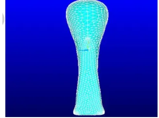
FEA mesh model with femur surface and attached ACL ligament. The femur surface is the upper part of knee joint which is considered for the data acquisition and segmentation and geometry construction. The ligament is inserted in the femur part. It is an approximate geometry, where the midsection cross-sectional area is smaller than that of the insertion. A typical ACL is comprised of bundle of collagen fiber, but the model used here is solid model with anisotropic material properties.

Figure 5: FEA Meshed Model of Ligament Figure 6: ACL Ligament Meshed Model

(5)

IJEDR1602063

351

IV. MATERIAL PROPERTY

Viscoelasticity

The shape of the stress-strain curve depends on the material itself and the test condition. However when the loads are applied and removed slowly, certain features of the stress-strain curve is similar for all structure materials. For example if the load is sufficiently small, the relation between stress and strain is linearly elastic. The material that behaves in a plastic manner does not retain to an unstrained state after the load is released. If after the load removal material response continues to change with time its response is said to be Viscoelastic or Viscoplastic. On removal of load, the stress-strain response of viscoelastic material follows a path (AB) that is different from the loading path. But in time after complete unloading the material will return to an unstrained state (along BO).

Figure 7: Nonlinear Elastic, Plastic and Viscoelastic Response

Table 1. Material Properties

Anisotropic Hyperelastic Material Properties

a1 1.5 MPa

C1 4.39056 MPa

C2 12.1093

D 0.001 MPa-1

Viscoelastic Material Properties

α1G 0.3

τ1G 0.3 sec

α2G 0.4

τ2G 0.9 sec

V.ELEMENT DESCRIPTION

Solid 187 have been used in order to mesh the Ligament model. it is higher order 3-D ,10 node element. It has quadratic displacement behavior and it is well suited for modeling irregular meshes. The element is defined by 10 nodes having 3 degree of freedom at each node: translation in nodal x, y, and z direction. The element has plasticity, hyperelasticity, large deflection and large strain capabilities. It also has mixed formulation capability for simulating deformation of nearly incompressible elastoplastic material, and fully incompressible hyperelastic material.

The geometry, nodes location and the coordinate system is shown in the below figure. In addition to the node the element data includes the orthotropic or anisotropic material properties. Orthotropic or anisotropic material direction corresponds to the element coordinate directions.

(6)

IJEDR1602063

352

VI. BOUNDARY CONDITION

A. Normal Flexion

The below figure shows the boundary conditions for normal flexion analysis where upper part is fixed and the tensile load is applied on the bottom part of ligament.

Figure .9: Normal Flexion Load B. 450_Flexion

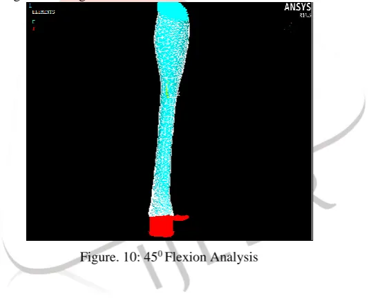
The below figure shows the condition for 45 degree flexion analysis.The upper part is kept fixed and the lower part of the knee joint has given load at an angle of 45 degrees.

Figure. 10: 450 _{Flexion Analysis}

VII. ANALYSIS

Assumption:

1) The ligament is fully developed without rupture. TheCAD model obtained from scanning is perfect modelling without any discontinuity.

2) The CAD model is meshed with the higher order solid element (solid 187). 3) The load acting on ligament is only in one direction. Other forces are neglected. 4) Material behavior is same like ligament.

5) Volume of the model is increase by the percentage over all dimensions.

Nonlinear Static Analysis

Nonlinear static analysis is performed under axial loading, bending and twist. Large deflection effects are included in this analysis. Because the purpose of this problem is to show the anisotropic, hyperelastic, and viscoelastic behaviour of the ACL ligament, a simplified model is used. Theproblems focus on the ACL part only. Instead of using complex model of ligament and femur only ligament is consider for analysis, remaining part is replace by the boundary conditions.

The femur part is kept fix and constrained with all degree of freedom the load is applied on the tibia part to perform analysis. The knee joint is work under flexion, extension and rotation therefore show the behavior of ACL under flexion, extension and rotation.

(7)

IJEDR1602063

353

The Femur part is fixed and normal load is applied on the tibia side. Four cases are considered for the analysis. The result is captured as an image for the first condition. The following images show the deformation, Von Mises stress, and elastic strain for the normal flexion analysis.

Figure. 11 Deformation Of Ligament Under Normal Flexion Figure. 12: Von Mises Stress of Ligament under Normal Flexion

In the above picture the deformation shows at the tibia side where the forces are applied.

Figure.13: Elastic Strain of Ligament Under Normal Flexion Figure. 14 Deformation of Ligament Under 450_Flexion

B. 450_{Flexion analysis}

(8)

IJEDR1602063

354

Figure.15:Von Mises Stress of Ligament under 450_{Flexion Figure.16 Elastic Strain of Ligament under 45}0_Flexion

VIII.RESULTANDDISCUSSION

Result Obtained After Nonlinear Static Analysis

After solving all the cases for flexion and rotation for ligament, the stress-strain relationship has studied for the behaviour of ligament. Because the ACL transmits tensile forces experimental studies of this tissue are generally performed in uniaxial tension.

A. Flexion analysis

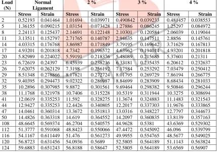
Table 2: Determination of Stress-Strain by Various Cases of Ligament Under Normal Flexion.

Load (N)

Normal Ligament

2 % 3 % 4 % Stress Strain Stress Strain Stress Strain Stress Strain

2 0.52193 0.041464 1.01694 0.039971 0.490842 0.039233 0.481457 0.038553 5 1.36155 0.090215 1.03154 0.073428 1.27886 0.086245 1.25297 0.084972 8 2.24113 0.125437 2.14691 0.122148 2.10301 0.120584 2.06039 0.119044 11 3.13511 0.152797 2.71765 0.140787 2.94635 0.147511 2.8856 0.145761 14 4.03315 0.176768 3.86987 0.171849 3.79195 0.169642 3.71629 0.167813 17 4.93201 0.201818 4.7342 0.196572 4.63962 0.194014 4.93201 0.201818 20 5.82989 0.224022 5.59191 0.218376 5.48089 0.215685 5.37601 0.21311 23 6.72619 0.24397 6.45939 0.238236 6.33181 0.235435 6.20612 0.232637 26 7.62075 0.262129 7.3198 0.256192 7.17584 0.253292 7.03479 0.250412 29 8.51348 0.278866 8.17821 0.272724 8.01795 0.269729 7.86194 0.266775 32 9.40395 0.294473 9.02322 0.286987 8.84699 0.283909 8.68434 0.281033 35 10.2896 0.307985 9.8872 0.301561 9.69464 0.298382 9.50846 0.296244 38 11.1768 0.321978 10.7406 0.315228 10.5319 0.311944 10.3275 0.308694 41 12.0619 0.335253 11.592 0.328275 11.3674 0.324883 11.1483 0.321543 44 12.9427 0.335253 12.4426 0.340805 12.2017 0.337303 11.9676 0.333865 47 14.0461 0.360314 13.3672 0.351813 13.0316 0.348227 12.7797 0.344673 50 14.4826 0.363318 14.619 0.364552 14.2097 0.360835 13.8139 0.357163 108 48.6645 0.569374 46.2704 0.540575 44.9628 0.5381 43.6369 0.529302 112 51.3777 0.591068 48.8423 0.550066 47.4472 0.545092 46.096 0.539799 116 54.1167 0.611449 51.476 0.561273 49.9955 0.554765 48.5677 0.549025 120 56.8723 0.631456 54.0936 0.5689 52.5805 0.564189 51.1143 0.563824 124 59.6883 0.651243 56.8188 0.58647 52.5805 0.564189 53.6569 0.56907

Above table shows the analysis for the normal flexion. The Load, Von misesstress, and Elastic strain are calculated for different loading condition. Four models are considered for the analysis. The result shows 2%, 3%, and 4% analysis results followed by normal ligament.

(9)

IJEDR1602063

355

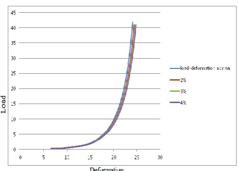
Figure. 17: Stress Vs Strain Relation Considering all Cases under Normal Flexion.

Figure.18: Load VsDeformation Relation Considering all Cases under Normal Flexion.

Above figure shows the effect of normal ligament and the percentage increased volume ligament for the same loading condition. Colour graph clearly shows the difference between each ligament values.

450_{Flexion Analysis}

Table 3: Determination of Stress-Strain By Various Cases of Ligament Under 450_Flexion

Load(N) Normal ligament 2 % 3% 4% Stress strain Stress strain Stress strain stress strain

0.25 0.609984 0.0501 0.593629 0.048559 0.585582 0.047801 0.577677 0.04706 0.5 0.936313 0.084637 0.916026 0.082297 0.906124 0.081151 0.896352 0.080028 2 3.25954 0.202152 3.14136 0.19817 3.08254 0.195247 3.02086 0.193961 6 9.92626 0.365568 9.57775 0.357095 9.39136 0.352908 9.2152 0.348005 26 39.1828 0.705994 37.9836 0.696079 37.3334 0.692025 36.7077 0.687459 29 43.1477 0.729021 41.7563 0.720897 41.0789 0.716304 39.3909 0.71204 32 47.0574 0.750508 45.5424 0.742128 44.774 0.737853 44.0224 0.733645 35 50.9284 0.769704 49.2762 0.761458 48.4361 0.757267 47.6192 0.753107 38 54.8133 0.786927 53.0023 0.778722 52.0949 0.77483 51.1859 0.770665 41 58.6467 0.803625 56.6853 0.795493 55.6734 0.791502 54.7596 0.791659

Above table shows the analysis for the 45 degree flexion. The Load, Von-mises stress, and Elastic strain are calculated for different loading condition. Four models are considered for the analysis. The result shows 2%, 3%, and 4% analysis results followed by normal ligament.

(10)

IJEDR1602063

356

Figure 21: Load V/S Deformation Relation Considering All Cases under 450_Flexion.

Discussion

The output obtained from model analysis is stress-strain and load-deformation. There are four results are obtained from each particular case. In order to obtained performance of ligament comparison of normal ligament with the percentage increased volume ligament carried out. Our aim is to achieve increase in performance of the ligament by increasing the volume of ligament.

1) In the model (Fig.No.11, 14) the peak stress in the ACL ligament are seen in the middle. Suggesting that this area could be susceptible to injury when the loading conditions are normal.

2) ACL can be injured or torn in a number of different ways. Some of the common ways are flexion and internal rotation of femur and tibia. During knee flexion increase in Von-misses stresses occurs near to the minimum cross sectional area. The stress in the ligament increases with the increase in internal rotation.

3) As the volume of the ligament increases the strain in the ligament decreases with the fewer amounts. The stress-strain curve shows nonlinearity within starting. So in order to increase performance volume increase will not be efficient.

4) Load - Deformation relation for the normal flexion analysis is same for all the ligaments. Therefore increase in volume does not effect on the deformation of the ligament in the case of 45 degree flexion analysis the deformation is increasing slightly.

5) For the 45 degree analysis the tibia side rotates and the femur remains fixed. During flexion an increase in Von-mises stresses occurs near the minimum cross sectional area of the ACL. The femoral and tibial insertion zones are not consider, as this model emphasis only the ACL part behaviour irrespective of insertion zones. If one also considers the insertion part, more accurate stresses near the femoral insertion zone can be expected.

IX. CONCLUSIONS

As the study shows, a ligament model can be analyzed for such conditions. The results clearly shows the effect of Stress - Strain relation when the loads are applied on the increased volume ligament. For the normal flexion near about 21 analyses are done with increased loading conditions and the graph for normal ligament showing triphasic behavior. The study of this paper is to understand the ligament behavior and the same result were obtained to conclude the result. For the 45 degree flexion the stress level matches with the normal flexion at very small load comparatively. There is a chance of ligament failure if the load is act on the knee while lower leg is at 45 degree.

A stress value reduced with the increasing volume of ligament and minimizes deformation and strain in all the two cases.The increase in volume of the ligament can increase the load carrying capacity of the body but the effect on the Stress-Strain shows less improvement compare with the normal values. To increase the ligament volume, the cost of the ligament will be very high when compared with the respected stress-strain effect. By increasing the volume of the ligament it is seen that performance of the ligament remains same. Therefore the increase in volume will not improve the load carrying capacity effectively.

X. ACKNOWLEDGMENT

The authors would like to thank Mr. Vinaay Patil for his assistance in material modeling.

REFERENCES

[1] Kiapour Ata M., KaulVikas, Kaipour Ali, Quatman Carmen E., Wordman Samuel C., Hewett Timonthy, Goel Vijay K., “The effect of ligament model technique on knee joint kinematics, a finite element study”. Applied mathematics 2013.

[2] Hosseini Ali, Gill Thomas J, Li Guan. “Estimation of vivo ACL force changes in response to increase weight bearing.” [3] Dai Boyi, Yu Bing. “Estimating ACL forces from lower extremity kinematics and kinetics”.

[4] Pena E., Calvo B., Martinez M.A., Doblare M. “An unisotropicvisco-hyperrelastic model for ligament at finite strains. Formulation and computational aspects”. International journal of solid and structure 44(2007).

(11)

IJEDR1602063

357

[6] Weiss A. Jeffrey, Gardiner John C, Ellis Benjamin J, Lujan Trevor J, Pahtak Nikhil S. “Three dimensional finite element

modeling of ligaments: Technical aspects”. Medical engineering and physics 2005.

[7] Song Yuhana, Debeski Richard E., MuashiVolkar, Thomas Maribeth, Savio L-Y. Woo “A three dimensional finite element model of the human anterior cruciate ligament: a computational analysis with experimental validation.” Journal of biomechanics 2004.

[8] Savio L. –Y. Woo, Steven D. Abramowitch, Robert Kilger, Rui Liang “ Biomechanics of knee ligaments: injury, healing, an repair” Journal of biomechanics 39 (2006) 1-20

[9] HirokawaShunji, Tsuruno Reiji. “Three-dimensional deformation and stress distribution in an analytical/computational model of anterior cruciate ligament” Journal of biomechanics 33 (2000) 1069-1077

[10]Kevin B. Shelburne, Marcus G. Pandy, Frank C. Anderson, Michael R. Torry “ Pattern of anterior cruciate ligament force in normal walking” Journal of biomechanics 37 (2004) 797-805

[11]G. Limbert, M. Taylor, J. Middleton “Three-dimensional finite element modeling of the human ACL: simulation of passive knee flexion with a stressed and stress-free ACL” Journal of biomechanics 37(2004) 1723-1731

[12]Bowman Jr. Karl F. Sekiya John K, “Anatomy and Biomechanics of the posterior cruciate ligament and other ligaments of the knee.” Journal of biomechanics (2009) 126-134