Compton Scattering Program Studying Nucleon Polarizabilities

Compton Scattering Program Studying Nucleon Polarizabilities

PhilippeMartel1,2,_,MaikBiroth1_{,CristinaCollicott}1,3,4,5_{,DilliPaudyal}6_{,andAliRajabi}7

onbehalfoftheA2collaborationatMAMI

1_{Institut für Kernphysik, Universität Mainz, D-55099 Mainz, Germany}

2_{Department of Physics, Mount Allison University, Sackville, New Brunswick E4L 1E6, Canada} 3_{Department of Physics, The George Washington University, Washington, D.C. 20052, USA}

4_{Department of Physics and Atmospheric Science, Dalhousie University, Halifax, Nova Scotia B3H 4R2, Canada} 5_{Department of Astronomy and Physics, Saint Mary’s University, Halifax, Nova Scotia B3H 3C3, Canada} 6_{Department of Physics, University of Regina, Regina, Saskatchewan S4S 0A2, Canada}

7_{Department of Physics, University of Massachusetts Amherst, Amherst, Massachusetts 01003, USA}

Abstract.The A2 collaboration at the Mainz Microtron has undertaken a program of Compton scattering

exper-iments with the goal of extracting the proton and, in the future, neutron polarizabilities. These are fundamental parameters that describe the response of the nucleon to an electromagnetic field. An extraction of these param-eters will provide a crucial test of QCD theories. This talk presented the concept and status of this program, including some preliminary results.

1 Introduction

Nuclear Compton scattering, the interaction of an electro-magnetic wave with a nucleon, can be described by a set of effective Hamiltonians. At lowest order this interaction is solely dependent on the mass,m, and electric charge,e, of the nucleon through

H(0)eff = π

2

2m+eφ, (1)

whereπ=p−eA. At the next order, the anomalous mag-netic moment,κ, becomes relevant in

He(1)ff =−e (1+κ)

2m σ·H− e(1+2κ)

8m2 σ·

E×π−π×E (2)

These first two orders encompass what are called the ‘Born’ terms, describing a point-like charged particle without internal structure.

1.1 Scalar Polarizabilities

As one goes to higher energies, the internal structure of the nucleon becomes evident by

H(2)eff =−4π

1 2αE1E

2₊1

2βM1H

2

, (3)

whereα_E1andβM1, so called scalar polarizabilities,

rep-resent the response of the nucleon to an applied electric or magnetic field, respectively. These effects can be visu-alized by imagining the nucleon being placed in a static field, as shown in Fig. 1. The application of an

_{Speaker - e-mail: [email protected]}

π+

π+

π+ π+

π+

π+

u

d u

π+

π+

π+

π+

π+

π+

π+ π+

u

d u

π+

π+

π+

π+

π+ π+

π+

π+

u

d u π+

π+

π+

π+

π+

π+

+ + + + + + +

− − − − − − −

++ ++

− −− −

E

π+ _u π+

d u

π+

π+

N N N N N NN S S S S S S SS

NNN N SSS

S

H Paramagnetic

Diamagnetic

Figure 1. Simplistic visual representation of the response of a

nucleon to an applied electric (left) or magnetic (right) field.

tric field causes a current within the pion cloud, eff ec-tively ‘stretching’ the nucleon. The application of a mag-netic field causes both a diamagmag-netic moment within the pion cloud and a paramagnetic moment in the constituent quarks. Though the scalar polarizabilities for the pro-ton have been determined through various Comppro-ton scat-tering experiments [1], some recent studies [2][3] have caused the Particle Data Group (PDG) to adjust the

viously quoted numbers [4]. Additionally, there is still interest in reducing the errors on these two factors, with the current values ofα_E1 = (11.2±0.4)×10−4fm3and

βM1=(2.5±0.4)×10−4fm3[5].

1.2 Spin Polarizabilities

For interactions at increasingly higher energies, the re-sponse of the nucleonspinto an electric or magnetic field begins to contribute through

He(3)ff =−4π

₁

2γE1E1σ·(E× ˙

E)+1

2γM1M1σ·(H× ˙

H)

−γM1E2Ei jσiHj+γE1M2Hi jσiEj

. (4)

The fourγfactors, called the spin polarizabilities, depict the response to an excitation by an electric or magnetic dipole (E1 or M1) or quadrupole (E2 or M2) followed by a de-excitation by an electric or magnetic dipole. Unlike the scalar polarizabilities, there had been no experimental determination of the values, other than several linear com-binations of them such as the forward spin polarizability

γ0=−γE1E1−γE1M2−γM1E2−γM1M1, (5)

for whichγ0 =(−1.0±0.08)×10−4fm4[6][7], and the

backward spin polarizability

γπ=−γE1E1−γE1M2+γM1E2+γM1M1, (6)

for whichγπ =(8.0±1.8)×10−4_fm4_{[8]. With the use}

of these two relations, one can change to a basis ofγ_E1E1,

γM1M1,γ0, andγπ, the use of which will be demonstrated in Sec. 4.

Though limited in experimental numbers, there have been various theoretical calculations and predictions of the spin polarizabilities, as given in Table 1. To address this

K-mat. HDPV DPV Lχ HBχPT BχPT

γE1E1 −4.8 −4.3 −3.8 −3.7 −1.1±1.8 −3.3 γM1M1 3.5 2.9 2.9 2.5 2.2±0.71 3.0 γE1M2 −1.8 −0.02 0.5 1.2 −0.4±0.4 0.2 γM1E2 1.1 2.2 1.6 1.2 1.9±0.4 1.1 γ0 2.0 −0.8 −1.1 −1.2 −2.6 −1.0

γπ 11.2 9.4 7.8 6.1 5.6 7.2

need for experimentally extracted spin polarizabilities, as well as improved scalar polarizabilities, the A2 collabora-tion at the Mainz Microtron (MAMI) facility, located in Mainz, Germany, began a program of Compton scattering experiments to investigate the proton polarizabilities. This

1_{Note in additional to the theory error given, there’s an additional} error onγM1M1of 0.5, as described in the paper [3].

program utilized polarized photon beams with both polar-ized and unpolarpolar-ized proton targets to measure the unpo-larized cross section as well as three asymmetries

Σ2x/z= NR

x/z−NLx/z PγPTNR_x/z+NL_x/z , Σ

3= N−N⊥ Pγ(N+N⊥). (7)

The first two of these asymmetries rely on a circularly po-larized photon beam and a transversely or longitudinally polarized proton target, respectively, where N_xR_//_zL repre-sents the number of events with x/z target polarization andR/Lbeam helicity,Pγrepresents the magnitude of the

beam polarization, andPTrepresents the magnitude of the target polarization. The third relies on a linearly polar-ized photon beam on an unpolarpolar-ized proton target, where

N/⊥represents the number of events with/⊥beam

po-larization, andPγrepresents the magnitude of the beam polarization.

2 Experiment

2.1 Beam

The MAMI facility is a cascade of racetrack mi-crotrons which can accelerate electrons up to energies of 1.6 GeV [15], with the additional capability of polarizing the beam longitudinally to a high degree [16]. The A2 hall is a real photon facility in which the electron beam strikes a thin radiator, producing Bremsstrahlung photons. The choice of a diamond radiator produces linearly polar-ized photons through coherent Bremsstrahlung, whereas an amorphous radiator combined with a longitudinally po-larized electron beam produces circularly popo-larized pho-tons through a helicity transfer process. The residual elec-tron is bent in a large spectrometer magnet into an array of 352 scintillators, permitting the tagging of the photon and determination of its energy with a resolution dependent upon the electron beam energy [17]. The photon beam is then collimated before intersecting with the target.

2.2 Targets

For measuringdσ0/dωandΣ3, an unpolarized liquid

hy-drogen target is sufficient. ForΣ2xandΣ2z, however, a

tar-get of polarized protons is required. This is accomplished with a Frozen Spin Target (FST) [18] through the process of Dynamic Nuclear Polarization [19]. The process be-gins by cooling the target to approximately 0.2 K and us-ing a large dipole magnet to align the electron spins. The polarization is then transferred to the proton by injecting microwaves at the appropriate frequency to cause spin-flip transitions. Once the desired polarization is achieved, the target is further cooled to about 25 mK in order to ‘freeze’ the spins in place. Even at this temperature, the target would still depolarize in a few hours without a field. To make room for the detectors, however, the polarizing mag-net needs to be removed, at which point a weaker holding coil is energized to maintain the polarization. The Mainz FST has been online since 2009, achieving polarizations up to 90%, with relaxation times of over 1000 h.

Table 1.Spin polarizabilities, in units of 10−4_fm4_{, K-matrix}

calculation [9], dispersion relation calculations HDPV [10] and DPV [11][12], chiral Lagrangian calculationLχ[13], heavy

Free radicals are needed in the FST in order for it to polarize, which necessitates the target material to be com-posed of more than just hydrogen. While several options are available, the Mainz group has opted to work with bu-tanol, C4H9OH. This does complicate the analysis due to

the inclusion of carbon and oxygen in the target, as well as the helium bath used to cool it down. A special carbon target was manufactured such that it could be inserted into the same cryostat, and run as a separate beamtime, to sub-tract out the contribution of the non-hydrogen nuclei in the butanol target.

2.3 Detectors

To analyze the final state of the interaction, a nearly 4π de-tector system is put in place over the target. This dede-tector system is composed of the Crystal Ball (CB) [20] and Two Arms Photon Spectrometer (TAPS) [21] systems. The CB is an array of 672 NaI crystals, covering 20◦ < θ <160◦

and−180◦ < φ < 180◦. This is coupled with a barrel

of 24 plastic scintillators called the Particle Identification Detector (PID), as well as a pair of Multi-Wire Propor-tional Chambers (MWPC), for charged particle identifi-cation and tracking [22]. TAPS is a vertical wall of 384 BaF2 and 72 PbWO4 crystals, which covers the

down-stream hole of the CB. It has an additional wall of plastic scintillators for charged particle identification. This sys-tem is shown in Fig. 2.

CB

NaI PID MWPC

Target TAPS

BaF2 PbWO4

Figure 2.Combined CB/TAPS detector system.

3 Analysis

A Compton scattering event is identified in the analysis by selecting final states where a single neutral track and a sin-gle charged track are detected. Coincidence between the time of the neutral track and the time of a hit in the tag-ger allows for tagging the initial state photon. In a high flux environment, however, the tagger experiences a large amount of accidental coincidences, for which a sideband subtraction is necessary, as shown in Fig. 3. The charged track time is not utilized in the accidental subtraction due

Tagger - Neutral Time (ns) 400

− −200 0 200 400 600

Counts

0 1 2 3 4 5 6 7 8 9

6

10

×

Figure 3.Timing difference between a neutral track and a hit in

the Tagger. The sharp ‘prompt’ peak at zero sits on a large acci-dental background which is removed by integrating two sideband regions, shown in red, and subtracting it from the integration of the prompt region, shown in green, after scaling by the ratio of the widths of these regions.

to the Time of Flight (TOF) experienced by the heavier proton. While the distance from the target center to the center of a NaI crystal in the CB is only 45 cm, TAPS is three to four times that distance from the target center, de-pending on the inclusion of a Cherenkov detector. Protons detected in TAPS, a large fraction of the phase space in this analysis, therefore exhibit a notable TOF. As noted in Sec 1, the spin polarizabilities play larger roles at higher energies; unfortunately extraction of these parameters at higher energies is more problematic, notably as more re-action channels open up. A compromise of measuring just below the two-pion photoproduction threshold (308 MeV) was taken, and an additional cut is made on tagger chan-nels within the region of interest.

Assuming an incoming photon with four-momentum

qi =(Ei, pi) strikes an at rest protonki=(mp,0,0,0) and results in a scattered photonqf =(Ef, pf), the ‘missing’

four-momentum is thenkf =qi+ki−qf, and the missing

mass for this reaction can then be calculated via

mmiss=

(Ei+mp−Ef)2−(pi−pf)2, (8)

under whichmmiss= mpfor a Compton scattering event. While the detection of the proton is required, energy losses suffered by it before detection prevent a total missing energy calculation. These losses will be discussed in Sec. 4.4. Instead, the vector of the track is compared to the vector ofkf, and an opening angle cut on this greatly reduces background, notably from coherent and incoher-ent scattering on carbon, oxygen, and helium. Any re-maining background from these reactions is then removed by subtracting out the separate data with the carbon target mentioned in Sec. 2.2.

Given that neutral pion (π0_{photoproduction has a cross}

section about 100 times larger than Compton scattering in theΔ(1232) region, an appreciable background signal is generated by cases where one of the decay photons (π0_{→γγ) goes undetected, and in some kinematic regions}

sim-ulation, or directly through the data itself. Similar to the sideband analysis of the tagger accidentals, one can take neutral pion events, which are fully detected in the system, where one of the decay photons is close to the known holes in the detector phase space. By neglecting this photon and analyzing the other decay photon, and the recoil proton, as if they were a Compton scattering event, one can mimic the background in the missing mass distribution. This dis-tribution, along with the various backgrounds, is shown in Fig. 4.

Missing Mass (MeV) 850 900 950 1000 1050 1100 1150 1200

Counts

0 500 1000 1500 2000 2500 3000

Figure 4.Missing mass distribution showing the tagger

acciden-tal (light blue), carbon (dark blue), and neutral pion (magenta, red, and yellow) background contributions, leaving the Compton signal in green.

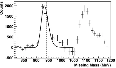
Subtracting out the various background contributions results in the distribution shown in Fig. 5. Missing mass distributions like this one are then integrated up to con-servative values near the proton mass, to ensure that any remaining neutral pion background is not included.

Missing Mass (MeV) 850 900 950 1000 1050 1100 1150 1200

Counts

-500 0 500 1000 1500 2000

Figure 5. Missing mass distribution after background

subtrac-tion, including a fit of the simulated line-shape.

4 Results

The A2 collaboration has completed its initial program of Compton scattering experiments with the goal of extract-ing the spin polarizabilities. The results, in some cases preliminary, are given below for each of the sub-projects.

4.1 _Σ2x: Transverse Target, Circular Beam

Measuring Σ2x required the use of the polarized target,

with the polarization direction transverse to the incom-ing beam of circularly polarized photons. The asymmetry was then constructed either by flipping the helicity of the photon beam, or by flipping the polarization of the target. While it takes roughly a day to flip the direction of the target polarization, the beam helicity is flipped regularly at a rate of about 1 Hz. This eliminates potential system-atic errors due to a change in detection efficiency between positive and negative target polarization data. However, to check such systematics, the target polarization was addi-tionally flipped, albeit only once or twice during a beam-time. The missing mass distributions for each helicity-polarization combination were integrated up to the proton mass, and then applied into Eq. 7, to produce the points shown in Fig. 6. This reflects data in the energy range of

Eγ=273−303 MeV [23].

(deg)

lab

θ

Compton 0 20 40 60 80 100 120 140 160 180

2x

Σ

-0.6 -0.4 -0.2 0 0.2 0.4 0.6

= 4.9

M1M1 γ

= 3.9

M1M1 γ

= 2.9

M1M1 γ

= 1.9

M1M1 γ

= 0.9

M1M1 γ

Figure 6. Σ2xforEγ=273−303 MeV. The theoretical curves

are from the HDPV dispersion code using different values for γM1M1as differentiated by color, whileαE1andβM1are assigned the PDG2012 values,γ0 =−1.0,γπ =8.0, andγE1E1=−4.3. The width of each band is generated by allowingαE1,βM1,γ0, andγπto vary by their experimental errors [23].

The curves shown in this figure were generated with the use of a dispersion relation code, provided by B. Pasquini [12]. The 2012 PDG numbers [4] were used for the initial scalar polarizabilities values, and the HDPV numbers [10], as shown in Tab. 1, were used for the initial spin polarizability values. In Fig. 6, the initial value for

γM1M1 was then perturbed by±1 and±2, in the standard

units, producing the different colored lines. The spread of each line reflects an additional step of allowingα_E1,

βM1,γ0, andγπ, to vary by their experimental errors, while keepingγE1E1fixed, and summing the resulting shifts in

quadrature. What Fig. 6 then depicts is a rough idea of the sensitivity of this asymmetry toγ_M1M1, which is clearly

small. Fig. 7 was constructed in a similar way except for varyingγE1E1and keepingγM1M1fixed instead. Here one

can see a much greater sensitivity to this particular spin po-larizability. With just this one observable, one can extract values ofγE1E1 =−4.6±1.6 andγM1M1=−7±11 [23].

Obviously the value forγM1M1is poorly fit, as predicted

(deg)

lab

θ

Compton 0 20 40 60 80 100 120 140 160 180

2x

Σ

-0.6 -0.4 -0.2 0 0.2 0.4 0.6

= -2.3

E1E1 γ

= -3.3

E1E1 γ

= -4.3

E1E1 γ

= -5.3

E1E1 γ

= -6.3

E1E1 γ

Figure 7.Σ2xforEγ=273−303 MeV. Similar to Fig. 6, except

nowγE1E1is allowed to vary, while one fixesγM1M1=2.9 [23].

in the fit by the four other polarizabilities. For these rea-sons, more data on different observables was required.

4.2 Σ3: Unpolarized Target, Linear Beam

While measuringΣ3only required the use of the simpler

unpolarized LH2target, it then required the use of a

di-amond radiator to generate a linearly polarized photon beam. The plane of polarization is adjustable, and was flipped by 90◦ roughly each hour. Instead of construct-ing the asymmetry by the events with each beam helic-ity, it was then determined by the polarization plane. The asymmetry was generated as a function ofφin addition to

Eγandθ. The distribution overφwas fit with a cos(2φ)

function, with the amplitude then representing the magni-tude of the asymmetry at thatEγandθ. This was done for two different energy ranges,Eγ=267.0−287.2 MeV and

Eγ=286.9−307.1 MeV, the latter of which is shown in

Figs. 8 and 9, with similar sensitivity curves as in Sec. 4.1.

(deg)

lab

θ

Compton 0 20 40 60 80 100 120 140 160 180

3

Σ

0.1

−

0 0.1 0.2 0.3 0.4 0.5

= 4.9

M1M1 γ

= 3.9

M1M1 γ

= 2.9

M1M1 γ

= 1.9

M1M1 γ

= 0.9

M1M1 γ

Figure 8. PreliminaryΣ3forEγ=286.9−307.1 MeV. Similar

to Fig. 6.

These results obtained at MAMI [24] complement those from a previous experiment at LEGS [25]. Each set ofΣ3data can then be taken with theΣ2xdata, from which

the polarizabilities can be fit while still utilizing the four constraints. The results of this inquiry are given in Tab. 2. The results from both MAMI and LEGS, for both energy ranges, are shown in Figs. 10 and 11. The theoretical

(deg)

lab

θ

Compton 0 20 40 60 80 100 120 140 160 180

3

Σ

0.1

−

0 0.1 0.2 0.3 0.4 0.5

= -2.3

E1E1 γ

= -3.3

E1E1 γ

= -4.3

E1E1 γ

= -5.3

E1E1 γ

= -6.3

E1E1 γ

Figure 9.PreliminaryΣ3forEγ=286.9−307.1 MeV. Similar

to Fig. 7.

Σ2xandΣLEGS3 Σ2xandΣ MAMI 3

¯

γE1E1 -3.5±1.2 -5.0±1.5

¯

γM1M1 3.16±0.85 3.13±0.88

¯

γE1M2 -0.7±1.2 1.7±1.7

¯

γM1E2 1.99±0.29 1.26±0.43

γ0 -1.03±0.18 -1.00±0.18

γπ 9.3±1.6 7.8±1.8

¯

α+_β¯ _{14.0±0.4 13.8±0.4}

¯

α−_β¯ 7.4±0.9 6.6±0.7

χ2_{/dof 1.05 1.25}

curves using the values given by the respective fits are also shown in Figs. 10 and 11. Additionally, the theoretical

(deg)

lab

θ

Compton 0 20 40 60 80 100 120 140 160 180

3

Σ

-0.1 -0.05 0 0.05 0.1 0.15 0.2 0.25 0.3 0.35

0.4 LEGS

3 Σ

LEGS 3 Σ Fit

MAMI 3 Σ

MAMI 3 Σ Fit

HDPV PT χ B

Figure 10. PreliminaryΣ3forEγ = 267.0−287.2 MeV. The

open circle data are those taken at MAMI [24], while the closed square data are those from LEGS [25]. The black and blue curves represent fitting theΣ2xdata from MAMI along with theΣ3data from either MAMI or LEGS, respectively, as shown in Tab. 2. The red and green curves show the theoretical predictions from HDPV and BχPT, respectively.

curves from the HDPV and BχPT codes, using their val-ues from Tab. 1, are plotted in those figures, depicting a better relationship between the HDPV theory and the

fit-Table 2.Dispersion relation fitted toΣ2xalong with either

ΣMAMI 3 [24] orΣ

LEGS

(deg)

lab

θ

Compton 0 20 40 60 80 100 120 140 160 180

3

Σ

-0.1 -0.05 0 0.05 0.1 0.15 0.2 0.25 0.3 0.35

0.4 LEGS

3 Σ

LEGS 3 Σ Fit

MAMI 3 Σ

MAMI 3 Σ Fit HDPV

PT χ B

Figure 11.PreliminaryΣ3forEγ=286.9−307.1 MeV. Similar

to Fig. 10.

ted values fromΣLEGS

3 [25], and between the BχPT theory

and the fitted values fromΣMAMI

3 [24].

4.3 _Σ2z: Longitudinal Target, Circular Beam

Completing the picture, and aiding the extraction of the spin polarizabilities without the use of theγ0andγπ con-straints, requires an additional lever-arm. This was accom-plished in the form ofΣ2z, another polarized target

asym-metry. In this case, the polarization of the target is set longitudinally with respect to the incoming beam of cir-cularly polarized photons. These data are the most recent taken in this A2 Compton program, and as such are still in the process of being analyzed. Some preliminary asym-metry values are shown in Figs. 12 and 13, also for the en-ergy rangeEγ=273−303 MeV. They only include about half of the data taken, were analyzed with only rough cal-ibrations applied, and only use some average polarization values. As such, these will certainly change upon comple-tion of the analyses of Paudyal and Rajabi. However, from the preliminary values one can at least observe both rea-sonable agreement with the curves as well as indications of reasonably high constraining power of these data.

(deg)

lab

θ

Compton 0 20 40 60 80 100 120 140 160 180

2z

Σ

0.4

−

0.2

−

0 0.2 0.4 0.6 0.8 1

= 4.9

M1M1 γ

= 3.9

M1M1 γ

= 2.9

M1M1 γ

= 1.9

M1M1 γ

= 0.9

M1M1 γ

Figure 12.PreliminaryΣ2zforEγ=273−303 MeV. Similar to

Fig. 6.

4.4 Active Target

As noted in Sec. 3, these analyses suffer in the detection of the recoil proton to the degree that its energy can not

(deg)

lab

θ

Compton 0 20 40 60 80 100 120 140 160 180

2z

Σ

0.4

−

0.2

−

0 0.2 0.4 0.6 0.8 1

= -2.3

E1E1 γ

= -3.3

E1E1 γ

= -4.3

E1E1 γ

= -5.3

E1E1 γ

= -6.3

E1E1 γ

Figure 13.PreliminaryΣ2zforEγ=273−303 MeV. Similar to

Fig. 7.

be absolutely determined. The energy and angular phase space is also limited by the energy loss of the proton, as lower energy recoils will simply not be detected. This can be verified by determining the proton efficiency fromπ0

photoproduction, as shown in Fig. 14. This shows that the

Max Eff 0.59 Thresh 70.47

Proton Ek (MeV)

0 50 100 150 200 250 300

)

M

+N

C

’/(N

C

N

0 0.1 0.2 0.3 0.4 0.5 0.6 0.7 0.8 0.9

1 Max Eff 0.59

Thresh 70.47

Figure 14. Proton efficiency =NC/(NC+NM) for the frozen

spin target, whereNC is the number of reconstructedγp→π0p

events that have a charged particle which satisfies an opening angle cut,NCis the number of events that have a charged particle,

andNMis the number of events that missed the recoil particle.

threshold for detection in the FST, determined at the half-max of the distribution, is approximately 70 MeV, and by 50 MeV the efficiency is basically zero. The recoil proton energy for the Compton scattering phase space is shown in Fig. 15. With a threshold of 70 MeV, only the region in the upper right hand corner is accessible. For this reason it is difficult to go below 270 MeV or forward of 80◦. The case is only slightly improved for the LH2target, where the

threshold is about 50 MeV. To reach much lower energies, however, requires a different approach.

0 20 40 60 80 100 120 140 160 180 200

Beam Energy (MeV) 0 50 100 150 200 250 300 350 400 450

Compton Angle (deg)

0 20 40 60 80 100 120 140 160 180

Figure 15. Compton kinematics, showing the recoil proton

en-ergy as color gradients as a function of the Compton scattering angle and the incoming beam energy.

Figure 16.Schematic of the active target [26].

can detect recoil protons immediately after the reaction, but before they have lost energy traversing the target ma-terial, cryostat, and various other sections before reach-ing the main detector system. Such a system will en-able analyses at much lower energies, especially around theπ0_{photoproduction threshold. One can already}

ana-lyze the LH2target data in this region as, both below and

slightly above threshold, other reactions can be kinemati-cally separated from Compton scattering. With the polar-ized target however, as described in Sec. 3, the inclusion of non-hydrogen nuclei complicate things. With the de-tection ability of the active target, the dominant coherent background from these nuclei can be eliminated as the en-tire nucleus recoils, rather than individual protons. A first run with the active target, in a transversely polarized state, was performed in 2016, and the data is in the process of being analyzed. Two major achievements of this run are already evident however, the first being the detection of the scintillations within the target, and the second being the polarization of the target. This latter was clear from the NMR readings during polarization, but also confirmed in the analysis by looking at a simpleπ0_target

asymme-try, as shown in Fig. 17. The clear flip in the asymmetry between target polarization states proves the target was in-deed polarized. The asymmetry is small since the analysis had not factored in the actual value of the target polariza-tion, or removed contributions from the carbon which act to dilute the asymmetry.

4.5 Scalar Polarizabilities

In addition to studying the spin polarizabilities of the pro-ton, the A2 collaboration undertook to improve the

situa-Neutral Pion Phi (deg) 150

− −100 −50 0 50 100 150

)

-+N

+

)/(N

--N

+

(N

0.015

−

0.01

−

0.005

−

0 0.005 0.01 0.015

Figure 17.Preliminaryπ0_{target asymmetry from the active}

tar-get, with the black points from the positively polarized target and the red points from the negatively polarized target, along with fits to the respective data.

tion on the scalar polarizabilities. Initial studies, also of theΣ3observable with an LH2target, although at incident

photon energies below theπ0 _{photoproduction threshold}

have been recently published [27]. As noted in Sec. 4.4, Compton scattering events from LH2can still be analyzed

at these energies, despite the absence of recoil proton de-tection. These asymmetries are shown in Fig. 18, as pre-sented in the paper [27].

With these data, fits were performed in the BχPT [2][29][14] and HBχPT [3] frameworks, which led to magnetic polarizability values ofβM1 = 2.8₋+2₂._.3₁×

10−4_fm3

andβM1=3.7+₋2_2..5₃×10−4fm3, respectively [27].

These data represent a proof-of-principle run taken in June 2013. A longer run, with improvements in both the tag-ging system and the linear beam polarization stability, is planned for the second half of 2017. This run will pro-vide both a reduction in the asymmetry errors by a factor of about 3.5, and a set of cross section measurements, that together will enable a single extraction ofα_E1andβM1at

level of the PDG errors.

5 Conclusions

0.8 −

0.6 −

0.4 −

0.2 −

0 0.2 3

Σ

0.8 −

0.6 −

0.4 −

0.2 −

0 0.2

0 20 40 60 80 100 120 140 160 0.8

− 0.6 −

0.4 −

0.2 −

0 0.2

] ° [

γ

θ

Figure 18.Beam asymmetryΣ3for three energy ranges

(upper-most: 79−98 MeV, middle: 98−119 MeV, lowermost: 119− 139 MeV). The errors represent statistical errors, the red bars indicate the systematic error. Green dashed curve: BχPT cal-culation [2], magenta dashed-dotted: DR calcal-culation [28][11], blue dotted: HBχPT [3], all withαE1= 10.65×10−4fm3and βM1= 3.15×10−4fm3; brown solid: Born term (curves corre-spond to the central values of the shown energy bins) [27].

Acknowledgments

We wish to thank the accelerator group and operators of MAMI for their outstanding support; H.W. Grießham-mer, J.A. McGovern, V. Pascalutsa, B. Pasquini, and D.R. Phillips for theory support; and the Messina confer-ence organizers for the talk invitation.

References

[1] V. Olmos de Leon et al., Eur. Phys. J. A10, 207 (2001).

[2] V. Lensky and V. Pascalutsa, Eur. Phys. J. C65, 195 (2010).

[3] J.A. McGovern, D.R. Phillips, H.W. Grießhammer, Eur. Phys. J. A49, 12 (2013).

[4] J. Beringeret al.(Particle Data Group), Phys. Rev. D

86, 010001 (2012).

[5] C. Patrignaniet al.(Particle Data Group), Chin. Phys. C40, 100001 (2016).

[6] J. Ahrens et al. (GDH/A2), Phys. Rev. Lett. 87, 022003 (2001).

[7] H. Dutz, K. Helbing, J. Krimmer, T. Speckner, and G. Zeitleret al.(GDH), Phys. Rev. Lett.91, 192001 (2003).

[8] M. Camen et al. (A2), Phys. Rev. C 65, 032202 (2002).

[9] S. Kondratyuk and O. Scholten, Phys. Rev. C 64, 024005 (2001).

[10] B.R. Holstein, D. Drechsel, P. Pasquini, and M. Van-derhaeghen, Phys. Rev. C61, 034316 (2000). [11] B. Pasquini, D. Drechsel, M. Vanderhaeghen, Phys.

Rev. C76, 015203 (2007).

[12] D. Drechsel, B. Pasquini, and M. Vanderhaeghen, Phys. Rep.378, 99 (2003).

[13] A.M. Gasparyan, M.F.M. Lutz, and B. Pasquini, Nucl. Phys. A866, 79 (2011).

[14] V. Lensky and J.A. McGovern, Phys. Rev. C 89, 032202 (2014).

[15] K.-H. Kaiseret al., Nucl. Instrum. Methods Phys. Res., Sect. A593, 159 (2008).

[16] V. Tioukine, K. Aulenbacher, and E. Riehn, Rev. Sci. Instrum.82, 033303 (2011).

[17] J. McGeorge, J. Kellie,et al., Eur. Phys. J. A37, 129 (2008).

[18] A. Thomas, Eur. Phys. J. Special Topics198, 171 (2011).

[19] D. G. Crabb and W. Meyer, Annu. Rev. Nucl. Part. Sci.47, 67 (1997).

[20] A. Starostinet al. (CB), Phys. Rev. C64, 055205 (2001).

[21] R. Novotny, IEEE Trans. Nucl. Sci.38, 379 (1991). [22] C. M. Tarbert et al.(CB@MAMI/A2), Phys. Rev.

Lett.100, 132301 (2008).

[23] P.P. Martel, R. Miskimen,et al.(A2), Phys. Rev. Lett.

114, 112501 (2015).

[24] C. Collicott, Ph.D. thesis, Dalhousie University (2015).

[25] G. Blanpiedet al.(LEGS), Phys. Rev. C64, 025203 (2001).

[26] M. Biroth, P. Achenbach, E. Downie, and A. Thomas (A2), PoS PSTP2015, 005 (2015).

[27] V. Sokhoyan, E.J. Downie, E. Mornacchi, J.A. Mc-Govern, N. Krupina,et al.(A2), Eur. Phys. J. A53, 14 (2017).

[28] D. Drechsel, M. Gorchtein, B. Pasquini, M. Vander-haeghen, Phys. Rev. C61, 015204 (1999).