Supplementary material

Supplementary material

Mid-infrared Laser Spectroscopy Detection and

Quantification of Explosives in Soils Using Multivariate

Analysis and Artificial Intelligence

Leonardo C. Pacheco-Londoño 1,2,*_{, Eric Warren} 1_{, Nataly J. Galán-Freyle} 1,2_{, Reynaldo} Villarreal-González 2_{, Joaquín A. Aparicio-Bolaño} 3,4_{, María L. Ospina-Castro} 5_{, Wei-Chuan Shih} 6 _{and Samuel P.} Hernández-Rivera 1,*

1 _{ALERT DHS Center of Excellence for Explosives Research, Department of Chemistry, University of Puerto Rico,} Mayagüez, PR 00681, USA; [email protected](L.P.); [email protected] (N.G.);

[email protected] (E.W.)

2 _{MacondoLab, Universidad Simón Bolívar, Barranquilla, Colombia [email protected]}

(L.P.); [email protected] (N.G.);[email protected] (R.V.)

3 _{Department of Physics, Florida International, FL, USA; [email protected]}

4 _{Physics, Chemistry, Physics and Earth Sciences Department, Miami-Dade College, Kendall Campus, Miami, FL,} USA; [email protected]

5 _{Grupo de Investigación Química Supramolecular Aplicada. Programa de Química, Universidad del Atlántico,} Barranquilla, Colombia; [email protected]

6 _{Department of Electrical & Computer Engineering University of Houston, 4800 Calhoun Rd. Eng. Bldg. 1, Rm.} N308, Houston TX 77204-4005, USA; [email protected]

* Correspondence: [email protected]; Tel.: 787-265-5404; 787-832-4040, x-5458, X-2638 (S.H.) [email protected]; Tel.: +57-304-648-9549 (L.P.)

Table S1. Composition percent of soil (NAT-S) samples.

TGA H2O2

Method TDS

Total Analyses

water content 5.3% 5.3%

OM 4.1% 4.1%

non-volatile solids 85.6% 85.6%

volatile 5.0%

volatile + OM 9.1% 9.1%

SSW 13.1% 13.1%

non-soluble solids 77.4%

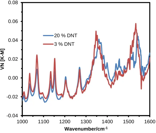
Figure S1. KM Spectra of 20 and 3 % of DNT from the NAT-S sample.

Figure S2. Vector Normalization of KM Spectra of 20 and 3 % of DNT from NAT-S sample.

0 1 2 3 4 5 6

1000 1100 1200 1300 1400 1500 1600

K

-M

Wavenumber/cm-1

20 % DNT

3 % DNT

-0.04 -0.02 0.00 0.02 0.04 0.06 0.08

1000 1100 1200 1300 1400 1500 1600

V

N

[K

-M]

Wavenumber/cm-1

20 % DNT

Figure S3. PLS models for DNT in KBr using VN prepossessing.

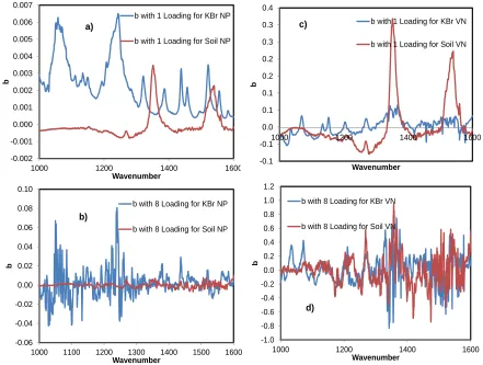
Figure S4. a) b regression vector for models without preprocessing and with one loading, b) b regression vector for models with vector normalization preprocessing and with one loading, c) b regression vector for models without preprocessing and with eight loadings, d) b regression vector for models with vector normalization preprocessing and with eight loading

-6 -1 4 9 14 19

0 5 10 15 20

Pr edict ed V alues (% )

Gravimetric Values (%) Val

Prediction

y = x

KBr [VN]

1000 1200 1400 1600

b

Wavenumber

b with 1 Loading for KBr NP

b with 1 Loading for Soil NP a) -0.06 -0.04 -0.02 0.00 0.02 0.04 0.06 0.08 0.10

1000 1100 1200 1300 1400 1500 1600

b

Wavenumber

b with 8 Loading for KBr NP

b with 8 Loading for Soil NP b) -0.1 -0.1 0.0 0.1 0.1 0.2 0.2 0.3 0.3 0.4

1000 1200 1400 1600

b

Wavenumber

b with 1 Loading for KBr VN

b with 1 Loading for Soil VN c) -1.0 -0.8 -0.6 -0.4 -0.2 0.0 0.2 0.4 0.6 0.8 1.0 1.2

1000 1200 1400 1600

b

Wavenumber

b with 8 Loading for KBr VN

b with 8 Loading for Soil VN

Figure S5. Plot of # of loading vs. analytical sensitivity for PLS models for DNT in KBr and Soil with VN preprocessing and without preprocessing.

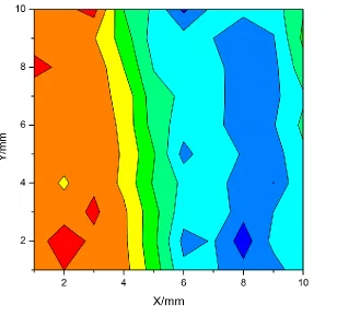
Figure S6. Map of % of DNT from NAT-S model (VN) of NAT-S-M sample.

0.0001 0.001 0.01 0.1

0 1 2 3 4 5 6 7 8 9



--1

(%

)

# Loading

DNT KBr NP

DNT Soil NP

DNT KBr VN

Figure S7. Map of % of DNT from NAT-S model (VN) of NAT-S-MM sample

Figure S9. Map of % of DNT from NAT-S model (VN) of NAT2-S sample

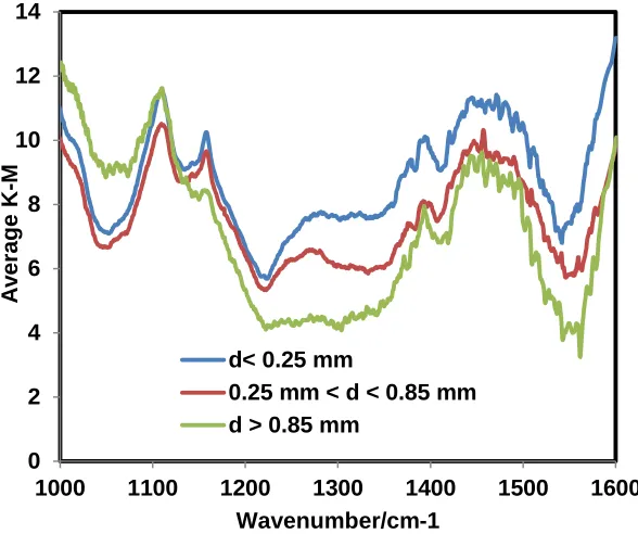
Figure S10. QCL Average spectra for different size of soil 0

2 4 6 8 10 12 14

1000 1100 1200 1300 1400 1500 1600

A

v

erage

K

-M

Wavenumber/cm-1 d< 0.25 mm

Figure S11. QCL spectra showing a standard deviation for various sizes of soil samples.

Figure S12. QCL average spectrum for various sizes of soil. 0.0

0.2 0.4 0.6 0.8 1.0 1.2 1.4 1.6 1.8 2.0

1000 1200 1400 1600

S

tan

da

rd

de

sv

iati

on

K

-M

Wavenumber/cm-1 d< 0.25 mm

0.25 mm < d < 0.85 mm d > 0.85 mm

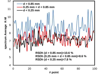
4 5 6 7 8 9 10 11 12

0 20 40 60 80 100

spectrum

A

v

er

age

K

-M

# point d > 0.85 mm

0.25 mm < d < 0.85 mm d < 0.25 mm

RSDh (d > 0.85 mm)=10.6 %

Table S13. Basic description of matching learning methods for classification [60]

ML METHODS DESCRIPTION

K-neighbors classifier(KNC)

Scikit-learn implements a K-neighbors classifier, a neighbors-based classification, where k is an integer value specified by the user. This is a type of instance-based learning or non-generalizing learning: it does not attempt to construct a general internal model, but simply stores instances of the training data. Classification is computed from a simple majority vote of the nearest neighbors of each point: a query point is assigned the data class, which has the most representatives within the nearest neighbors of the point.

SVC

Support vector machines for classification (SVC) is an algorithm capable of performing multi-class classification on a dataset. They are a set of supervised learning methods used for classification. These are based on the library (libsvm). In SVC, the fit time scales at least quadratically with the number of samples and may be impractical beyond tens of thousands of samples.

Decision Tree Classifier (DTC)

Decision Tree Classifier is a non-parametric supervised learning method is an algorithm capable of performing multi-class classification on a dataset. The goal is to create a model that predicts the value of a target variable by learning simple decision rules inferred from the data features. For instance, classical decision trees learn from data to approximate a sine curve with a set of if-then-else decision rules. The deeper the tree, the more complex the decision rules, and the fitter the model.

Random Forest Classifier (RFC)

Random forests classifier is an ensemble learning method for classification that operates by constructing a multitude of decision trees at training time and outputting the class that is the mode of the classes of

the individual trees. Random decision forests correct for decision trees’

habit of overfitting to their training set. A random forest is a meta estimator that fits several decision tree classifiers on various sub-samples of the dataset and uses averaging to improve the predictive accuracy and control over-fitting.

AdaBoost Classifier (ABC)

An AdaBoost[61] classifier is a meta-estimator that begins by fitting a classifier on the original dataset and then fits additional copies of the classifier on the same dataset but where the weights of incorrectly classified instances are adjusted such that subsequent classifiers focus more on severe cases. This class implements the algorithm known as AdaBoost-SAMME[61].

Gaussian Naive Bayes (GNB)

feature means and variance online, see Stanford CS tech report STAN-CS-79-773 by Chan, Golub, and LeVeque

Linear Discriminant Analysis (LDA)

Linear Discriminant Analysis, it is a classifier with a linear decision boundary, generated by fitting class conditional densities to the data and

using Bayes’ rule. The model fits a Gaussian density to each class,

assuming that all classes share the same covariance matrix. The fitted model can also be used to reduce the dimensionality of the input by projecting it to the most discriminative directions.

Quadratic Discriminant Analysis (QDA)

Quadratic Discriminant Analysis, it is a classifier with a quadratic decision boundary, generated by fitting class conditional densities to the

data and using Bayes’ rule. The model fits a Gaussian density to each