Article 1
A Controlled-Site Comparison of Microwave
2Tomography and Time-Reversal Imaging Techniques
3for GPR Surveys
4Vinicius Santos 1,*, Emerson Almeida 1, Jorge Porsani 1,Fernando Teixeira 2 and Francesco 5
Soldovieri 3 6
1 Universidade de São Paulo (USP), Instituto de Astronomia, Geofísica e Ciências Atmosféricas (IAG), 7
Departamento de Geofisica, SP/Brazil; [email protected] (E.A.); [email protected] (J.P.) 8
2 ElectroScience Laboratory and Department of Electrical and Computer Engineering, The Ohio State 9
University, Columbus, OH USA; [email protected] (F.T.) 10
3 IREA-CNR, Institute for Electromagnetic Sensing of the Environment, National Research Council of Italy, 11
via Diocleziano 328, 80124 Napoli, Italy; [email protected] (F.S.) 12
* Correspondence: [email protected]; Tel.: +55-11-3091-4734 13
Abstract: This paper provides a comparative study between microwave tomography and synthetic 14
time-reversal imaging techniques as applied to ground penetrating radar (GPR) surveys. The 15
comparison is carried out by processing experimental data collected at a controlled test site, with 16
various types of buried targets at given subsurface depths and representative soil conditions. It is 17
shown that the two techniques allow us to obtain complementary information about position, 18
depth and size of the targets from a single GPR survey. 19
Keywords: ground penetrating radar; microwave tomography; time-reversal technique 20
21
1. Introduction 22
Ground penetrating radar (GPR) finds a large number of applications related to detection and 23
imaging of subsurface targets and anomalies such as underground utilities, pipes, chemical spills, 24
groundwater levels, etc. Historically, GPR data has been typically analyzed and interpreted based 25
on a “visual” analysis of the radargram [1], [2]; however, this analysis is able to provide reliable 26
interpretation only in simple scenarios. In order to improve the interpretability of GPR data, inverse 27
scattering and migration algorithms [3]-[8], including microwave tomography (MT) techniques 28
[9]-[11], have also been used in different scenarios related to GPR surveys. MT has been successfully 29
used for example to investigate water leakage from a large metallic pipe in [12], where it was able to 30
give more reliable information than a direct radargram analysis. In addition, several GPR surveys at 31
different time intervals were done for a controlled oil spill and analysed through MT in [13]. 32
In all these scenarios, environmental clutter can affect the measured data and deteriorate imaging 33
results, making more difficult the estimation of the target geometry [14]. For imaging metallic and 34
plastic pipes, MT was compared to conventional migration techniques in [15] under controlled 35
experimental conditions, where it was shown that MT is capable of providing improved accuracy 36
and resolution. A similar study was carried out in [16] in a forensic application scenario. A 37
theoretical analysis of the reconstruction performance of the MT and migration was carried out in 38
[17] based on the Singular Value Decomposition of the relevant operator. MT also proved capable of 39
providing good results for multi-frequency systems [18]. The effect of background electrical 40
conductivity values on tomographic images was addressed [19]. This latter study showed that the 41
more accurate the estimated background conductivity value, the higher the contrast function image 42
sharpness associated with the anomaly of interest, suggesting that this effect can be alternatively 43
exploited to estimate the background medium conductivity as well. Structural degradation 44
assessment using a combination of MT and seismic tomography was discussed by [20] for cultural 45
heritage monitoring. 46
Finally, the flexibility enabled MT has permitted its use for processing data acquired from 47
airborne surveys [21], where it was shown that very good results can obtained, especially in areas 48
with no vegetation covers, such as glaciers. 49
Time-reversal-based (TR) techniques were first developed for acoustics [22], [23], and later 50
successfully used in several applications including medicine [24], [25], non-destructive testing and 51
evaluation [26], atmospherics studies [27], microwave remote sensing [28], as well as 52
near-subsurface geophysics [29]-[34]. As the name suggests, TR-based techniques exploit the 53
invariance of the wave equation under time reversal. The received data can be synthetically 54
time-reversed (in a first-in last-out fashion) and, after physical or synthetic re-transmission to the 55
region of interest, used to create wavefields that automatically focus on reflective targets and/or 56
anomalies. Under certain conditions, TR techniques can be used for detection and localization of 57
obscured targets in cluttered and rich-scattering environments. Variants on the basic TR algorithm 58
exist, which allow for selective focusing (on secondary or weaker targets) [35], [36] or tracking of 59
obscured moving targets as well [37]. 60
The objective of this work is to compare MT and TR by analysing reconstruction results obtained 61
by experimental data from GPR surveys on a controlled site with known subsurface targets. This 62
comparison has the objective to examine the relative weakness and strengths of each method under 63
conditions pertaining to realistic GPR field acquisitions. The consideration of a controlled site with 64
known targets allows for a better assessment of the capabilities and drawbacks of the two 65
approaches. It is worth noting that the test site is at the scale of the realistic conditions and is more 66
challenging than usual laboratory conditions. The targets under investigation are representative 67
examples of objects normally found in archaeological sites (disturbed soil and ceramic vases), 68
geotechnical evaluations (concrete tubes) and environmental surveys (storage tanks). The 69
comparison between MT and TR is presented here for the first time in literature and suggests that 70
the two approaches could be potentially used in a complementary fashion. 71
The paper is organized as follows. Sections 2 and 3 provide a brief overview of the MT and TR 72
methodologies, respectively. Section 4 describes the controlled site characteristics and the set of 73
buried target considered. Section 5 compares the results from experimental GPR data. Finally, some 74
concluding remarks are provided in Section 6. 75
76
2. Microwave tomography 77
Since both MT and TR have been widely studied in the past, we will only discuss them very 78
briefly here. 79
MT formulates the GPR data processing as an inverse scattering problem [38], [39]. Consider for 80
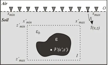
simplicity the 2D geometry depicted in Figure 1. Each triangle indicates the position of the 81
transmitter-receiver pair. In a common-offset GPR, each trace of the radargram is acquired at a 82
corresponds to the observation domain . The electric field irradiated by the transmitter antenna in 84
absence of targets corresponds to the incident field . The targets are assumed to be buried inside 85
the region on interest , which is discretized by a regular grid of points ′ ′, ′ . The interaction of a 86
buried target with the incident field generates the scattered electric field . The summation of 87
scattered and incident fields results in the total electric field . The scattered field on the 88
measurement domain conveys the information about the buried targets and represents the input 89
data to the processing scheme. According to [40] the scattered field can be written as 90
, = ̿ | ∙ ; ∈ (1)
where = − is the complex wavenumber of the background medium, is the 91
angular frequency, is the free-space magnetic permeability, is the dielectric permittivity, 92
is the electric conductivity and ̿ is the background Green’s function [40]. The contrast function 93
is the unknown of the tomographic imaging inverse problem and is defined as 94
= − 1 (2)
where ′ = ′ − ̅′ ⁄ is the dielectric permittivity inside the region of interest , 95
′ is the dielectric constant inside , and = − ⁄ is the dielectric permittivity of the 96
homogenous background medium. The problem in (1) is nonlinear. The most common linearization 97
strategy for this problem is to employ the Born approximation [40]. Under its assumptions, the total 98
field is approximated by the incident field in (1), so that the expression for the scattered electric 99
becomes 100
, ≈ ̿ | ∙ ; ∈ (3)
The problem stated by (3) is ill-posed, and stability of the solution is affected by the noise present 101
in the data. In order to achieve a stable solution, regularization schemes can use used. Here, we 102
adopt the Truncated Singular Value Decomposition (TSVD) [41]. The equation (3) can be written as 103
= ℒ[ ] where ℒ represents the linear operator connecting the contrast function to the scattered 104
field data. In the presented approach, ℒ is discretized using the method of moments [42]. By 105
applying a SVD on this linear operator, we can write 106
= 〈 , 〉 (4)
from which the solution for can be obtained by inverting (4), i.e., 107
= 〈 , 〉 (5)
where ∞ is the set of singular vectors (orthonormal basis) in the data space, ∞ is the set 108
of singular functions vectors (orthonormal basis) in the space of unknowns. ∞ is the set of 109
singular values ordered in a decreasing order, and is the truncation index. is a 110
problem-dependent parameter selected to achieve a good balance between resolution and stability 111
against noise [38], [39]. The truncation indexes used here are discussed in Section 5. 112
Figure 1. Problem geometry, see text for details. 114
115
3. Time-reversal-based technique 116
TR-based techniques were first introduced for ultrasonic waves [22], [23] and later extended to 117
electromagnetic waves. They explore the invariance of the wave equation under the time reversal 118
[43]. This invariance is only exact in reciprocal and lossless media; anyway, under certain conditions, 119
the techniques can be also applied to lossy media as well. In rich scattering scenarios, TR can achieve 120
super-resolution and for wideband signals, it can provide statistical stability for imaging in random 121
media [44]-[47]. The basic TR process is given by the following steps [43]: 122
(i) A short pulse is transmitted from one or more transceivers to the region of interest where it is 123
scattered by one or more targets; 124
(ii) The scattered signal is registered by the transceivers; 125
(iii) The received signal waveform is time-reversed (first-in, last-out) and retransmitted (either 126
physically or synthetically) to the region of interest; 127
(iv) Due to time invariance of the wave equation, the retransmitted waveform will tend to focus 128
around the original target location(s). 129
In the TR process, the focusing of the retransmitted waveform suffers of limitations in the 130
resolution, because the receivers typically comprise a limited-aspect aperture in practice (i.e., they 131
do not capture the scattered field in all directions), the evanescent spectrum (present only in the very 132
near-field) is not captured, and for the presence of losses, if any, in the region of interest. 133
Nevertheless, under some conditions [43], the resolution enabled by TR can go beyond the one 134
dictated by the conventional diffraction limit. The TR process can also be understood as a matched 135
filter operation in both time and space [43], [44]. Assuming that a transmitter at a location sends a 136
pulse s(t), the signal measured at a receiver located at can be expressed in terms of the 137
convolution1
138
= ∗ ℎ (6)
where ℎ is the impulse response (time-domain Green’s function) between and . From the 139
reciprocity theorem, we can write ℎ = ℎ , and the time-reversed retransmitted signal at 140
due to a source at is given by 141
= − ∗ ℎ − ∗ ℎ (7)
where − ∗ ℎ − is − . Generally, for a time reversal array (TRA) with N transceivers, 142
the received signal is given by the following equation 143
, = − ∗ ℎ − ∗ ℎ (8)
A more extensive discussion on TR-based techniques and their variants can be found in [43]. 144
145
4. Test site 146
The comparative study comprised eight different targets, representative of objects found in 147
archaeological, geotechnical, and environmental studies. The experimental data was collected at a 148
controlled test site (at the scale of the realistic situations) situated in the Institute of Astronomy, 149
Geophysics and Atmospheric Science at the University of Sao Paulo (IAG/USP), Brazil, see Figure 2, 150
during dry weather. The test site is situated at the border of a sedimentary basin in the southwest of 151
Brazil, characterized by clay soil and clay-sand sediments overlapped to a granite-gneissic basement. 152
The test site is outdoors and is affected by the climatic events. 153
154
(a)
(b)
Figure 2. a) Test site panoramic view. b) Acquisition on the test site with 200 MHz antenna. 155
156
A commercial 200 MHz GPR system manufactured by GSSI (Geophysical Survey Systems, Inc.) 157
was used to collect the data. We used 512 samples in each A-scan, 100 ns for the time-window and a 158
total of 50 A-scans/m of sampling. The GPR system employs shielded bow-tie antennas and has a 159
nominal frequency range from about 50 MHz to about 325 MHz. 160
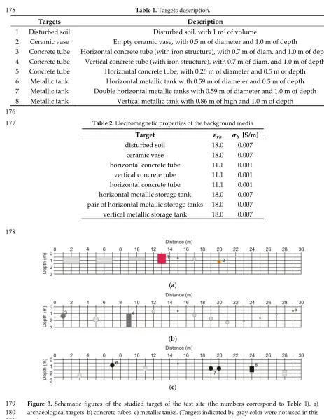
Table 1 provides the list of the targets present underneath each of the GPR tracks considered. 161
Figure 3 shows a schematic view of the target distribution in the subsoil. Before data processing by 162
either MT or TR, the acquired radargrams were pre-processed using ReflexWTM software [48] using a
163
conventional sequence based on header gain removal, zero-time correction, background removal, 164
gain function, and frequency filtering. Since the targets are buried at different locations in a wide 165
area, the background medium (soil) may exhibit some variation on its permittivity due to soil 166
content variations in shallow geologic material. Because of this, the (mean) permittivity was first 167
retrieved using the relation = ⁄ where is the speed of light and is the phase velocity 168
on the subsoil. The (mean) conductivity was also retrieved a priori, by analyzing the images after 169
performing the inversion with different conductivity values and selecting the value that gives the 170
better focused tomographic image. This procedure is similar to that described by [19]. The values 171
adopted for the electrical properties in subsoil are summarized in Table 2. 172
Table 1. Targets description. 175
Targets Description
1 Disturbed soil Disturbed soil, with 1 m3 of volume
2 Ceramic vase Empty ceramic vase, with 0.5 m of diameter and 1.0 m of depth
3 Concrete tube Horizontal concrete tube (with iron structure), with 0.7 m of diam. and 1.0 m of depth 4 Concrete tube Vertical concrete tube (with iron structure), with 0.7 m of diam. and 1.0 m of depth 5 Concrete tube Horizontal concrete tube, with 0.26 m of diameter and 0.5 m of depth 6 Metallic tank Horizontal metallic tank with 0.59 m of diameter and 0.5 m of depth 7 Metallic tank Double horizontal metallic tanks with 0.59 m of diameter and 1.0 m of depth 8 Metallic tank Vertical metallic tank with 0.86 m of high and 1.0 m of depth 176
Table 2. Electromagnetic properties of the background media 177
Target [S/m]
disturbed soil 18.0 0.007
ceramic vase 18.0 0.007
horizontal concrete tube 11.1 0.001 vertical concrete tube 11.1 0.001 horizontal concrete tube 11.1 0.001 horizontal metallic storage tank 18.0 0.007 pair of horizontal metallic storage tanks 18.0 0.007 vertical metallic storage tank 18.0 0.007
178
(a)
(b)
(c)
Figure 3. Schematic figures of the studied target of the test site (the numbers correspond to Table 1). a) 179
archaeological targets. b) concrete tubes. c) metallic tanks. (Targets indicated by gray color were not used in this 180
study) 181
5. Comparative results 182
MT has exploited a frequency bandwidth cited above, where a sampling was done with 19 183
in 0.025 m × 0.025 m pixels for all the considered cases. 185
For the MT results, the TSVD regularization parameter was chosen case by case according to the 186
best reconstruction; the values of the regularization parameters are listed in Table 3. The frequency 187
sampling was done with 19 frequencies equally distributed in the 50 MHz to 325 MHz bandwidth. 188
189
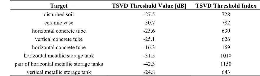
Table 3. Threshold values adopted for the TSVD regularization 190
Target TSVD Threshold Value [dB] TSVD Threshold Index
disturbed soil -27.5 728
ceramic vase -30.7 782
horizontal concrete tube -25.6 630
vertical concrete tube -25.1 626
horizontal concrete tube -16.3 169
horizontal metallic storage tank -31.5 1010
pair of horizontal metallic storage tanks -42.3 1150
vertical metallic storage tank -24.8 643
191
TR images can be obtained according to the procedure described in [33], [34] where the standard 192
deviation of the backpropagated TR wavefield amplitudes, sampled in either time or space (i.e. 193
depth or co-range), is used to provide the dispersion of each data set. In this manner, larger 194
variations in the TR amplitudes caused by focusing effects yielded the back-propagated field are 195
emphasized without the need for a precise a priori estimate of the focusing instant (as it turns out to 196
be necessary in other TR approaches). The standard deviation is computed for the whole data set, 197
comprising a three-dimensional TR matrix. After data acquisition, the TR retransmission step 198
(backpropagation) is carried out, as in any imaging application, synthetically. The FDTD 199
(finite-difference time-domain) algorithm [49] is employed here for this purpose. 200
In [33], [34] two types of data processing are applied for computation of the standard deviation, 201
denoted as Mode 1 and Mode 2. Mode 1 aims at emphasizing the cross-range resolution or the target 202
position along the GPR track, whereas Mode 2 tends to emphasize the co-range resolution or the 203
target depth. Although these modes provide data that can in principle be applied and interpreted 204
separately, the single mode results can be affected by spurious artifacts such as ringing effects that 205
can confound interpretation. In order to decrease the image artifacts and improve the results, we 206
exploit the best features of both modes in the present study, by combining their data based through a 207
cross-correlation (ccTR). In all of the presented results, the upper panel shows the conventional 208
radargram, the middle panel shows the image obtained MT, and the bottom panel shows the ccTR 209
image. White dashed lines indicate the geometric shape and actual location of each target. In all 210
results, each technique yield “artifacts” in the reconstructed images, in addition to the target 211
response. These anomalies (secondary reflections) are prevalent in most field data due to the 212
presence of geologic stratification and other inhomogeneities in the subsurface. The indication of 213
these artifacts in all three techniques is provided by red arrows. 214
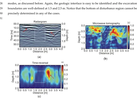
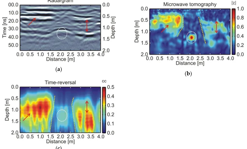
Target 1: Disturbed soil. Results from the processing of the GPR data acquired over the region 215
comprising a disturbed soil are shown in Figure 4. Figure 4a shows the pre-processed radargram, 216
by the dashed white rectangle indicating the region of disturbance. The reflection amplitudes are 218
reduced because any significant reflection to geological stratification was removed by the excavation 219
and refilling process. In particular, a strong reflector related to a shallow geologic interface is present 220
at a depth of about 0.5 m, beyond the 2.5 m position along the GPR line (indicated by red arrows). 221
This reflector appears at lower depths at the near end of the radargram and is interrupted by the soil 222
disturbance. Figure 4b shows the MT results. The strong responses in the region between the surface 223
and a depth of about 1 m are again associated to reflections caused by geologic stratification on the 224
test site. Although the discontinuity in the response does not reproduce the exact disturbance width, 225
the evidence of soil disturbance is also clear in this image, with a sharper delineation compared to 226
the radargram result. Figure 4c shows the image obtained based on cross-correlation of the two TR 227
modes, as discussed before. Again, the geologic interface is easy to be identified and the excavation 228
boundaries are well-defined at 1.5 and 2.5 m. Notice that the bottom of disturbance region cannot be 229
precisely determined in any of the cases. 230
231
(a)
(b)
(c)
Figure 4. Disturbed soil. a) Radargram. b) Microwave tomography image. c) Time-reversal data. The dashed 232
line rectangle indicates the actual target location. 233
234
Target 2: Ceramic vase. Figure 5 shows the results from GPR data for an investigation domain 235
containing a ceramic vase buried at a depth of 1.0 m. A shallow geologic interface at the depth of 236
about 0.5 m can be again discerned from the radargram shown in Figure 5a (indicated by red 237
arrows). There is also a clear reduction in the reflection amplitude above the target location, which 238
results from the soil excavation for burying the target. The anomaly related to the target appears as a 239
hyperbolic feature at the depth of about 1.0 m. However, this hyperbolic feature is merged to 240
another strong horizontal reflection at the depth of around 1.2 m, which is related to geological 241
geologic background. The discontinuity of the geologic reflectors is also evident, as indicated by the 243
dashed lines, and is indicative of the excavation done prior to target installation in the test site. The 244
delocalization in depth for the MT reconstruction can be explained as follows. Ceramic vase is a 245
low-loss dielectric object, therefore, electric field is able to penetrate into the object and this entails 246
the possibility that the tomographic approach is able to reconstruct both the upper and lower edges 247
of the target (see for example reconstruction in [56]). These two reconstructed edges are well 248
detected and visible in the tomographic image if the resolution along the depth is adequate. When 249
the resolution in depth is not adequate (as in the case at hand), the two spots accounting for the edge 250
combine and give the reconstructed spot at the center of the target. 251
The image obtained based on the ccTR is shown in Figure 5c. The excavation marks are defined 252
and the presence of geologic layers between the ground and a depth of 1.5 m is visible. In the target 253
location, we can see an anomaly with a good lateral delineation that the conventional radargram 254
result. In particular, the TR results can provide good estimates for depth, position along track, and 255
lateral extent of the target in this case. 256
257
(a)
(b)
(c)
Figure 5. Ceramic vase. a) Radargram. b) Microwave tomography image. c) Time-reversal data. The dashed line 258
circle indicates the actual target location. The vertical dashed lines are associated with the lateral boundaries of 259
the excavated zone. 260
261
Target 3: Horizontal concrete tube with 0.7 m diameter. Figure 6 shows the results from the GPR 262
survey over a horizontal concrete tube with 0.7 m of diameter. The radargram presented in Figure 6a 263
exhibits a clear hyperbolic anomaly related to the target at a depth of about 0.8 m. A strong geologic 264
reflector 0.6 m deep is also visible beyond 2.8 m position along the GPR track line (indicated by red 265
arrows). Part of this reflector is seen also between the 0.4 m and 1.25 m positions. The image 266
retrieved from the MT is shown in Figure 6b, where a strong anomaly related to the target is visible 267
close to the top of the true target position, as indicated by the dashed line circle, with a slight vertical 268
geologic reflector as indicated by the vertical dashed lines. The corresponding ccTR image is shown 270
in Figure 6c, where the anomaly exhibits a similar pattern to the previous cases but with a slight 271
deviation in depth. This may have been caused by the presence of the small anomalies seen above 272
the target. The lateral boundaries of the excavation region can be well discerned again. 273
274
(a)
(b)
(c)
Figure 6. Horizontal concrete tube ( = 0.7 m). a) Radargram. b) Microwave tomography image. c) 275
Time-reversal data. The white circle indicates the actual target location. The vertical dashed lines are associated 276
with the lateral boundaries of the excavated zone. 277
278
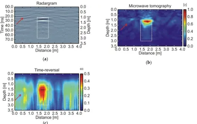
Target 4: Vertical concrete tube. Results corresponding to the vertical concrete tube are presented 279
in Figure 7. The response associated to this target is strong, but mostly confined to the top boundary 280
of the target (shallow end) due to the strong reflection and the fact that the field is not able to 281
penetrate into the metallic structure. The target response in the MT image presented in Figure 7b 282
arises from the top boundary (upper side) as well. The TR processing result is shown in Figure 7c, 283
which yields a good match for both the target position, as well as vertical and horizontal dimensions. 284
The top of the anomaly is rightly located and the bottom is clearly defined at 3.0 m approximately. 285
However, together with the target vertical extent recovery, secondary artifacts arise in other portions 286
of the image, associated with deeper geological features. 287
(a)
(b)
(c)
Figure 7. Vertical concrete tube. a) Radargram. b) Microwave tomography image. c) Time-reversal data. The 293
dashed line retangle indicates the target position. 294
295
Target 5: Horizontal concrete tube with 0.26 m diameter. Figure 8 shows the results for the GPR 296
survey over a horizontal concrete tube with 0.26 m of diameter. A clear hyperbolic anomaly is 297
present at the depth of 0.5 m in the radargram presented in Figure 8a. The correspondent 298
tomographic image in Figure 8b shows a strong anomaly coincident to the true target location. 299
Weaker anomalies related to the geologic background are indicted by the red arrows and exhibit a 300
spatial arrangement roughly delineating the lateral and lower edges of the excavation done for 301
target installation in the test site (dashed lines). Despite a visible anomaly associated with the 302
concrete tube, the ccTR result in Figure 8c does not show a good resolution for this particular target. 303
The anomaly has a circular shape and an amplitude close to that of the target. In this case, as visible 304
in all three results, there is a strong geological reflector at a location near 1.5 m along track and about 305
0.8 m in depth which can be confused with another target. 306
(a)
(b)
(c)
Figure 8. Horizontal concrete tube ( = 0.26 m). a) Radargram. b) Microwave tomography image. c) 313
Time-reversal data. The small circle indicates the actual target location. 314
315
Target 6: Single horizontal metallic storage tank. Figure 9 depicts the results from the GPR survey 316
over a horizontal metallic storage tank. A clear, well-defined hyperbolic anomaly is observed in the 317
radargram shown in Figure 9a at about 0.5 m in depth and 2.0 m along track. A horizontal reflection 318
trace related to a geologic interface is observed as well near 1.0 m deep (indicated by red arrows). 319
The image retrieved from MT in Figure 9b shows a single strong anomaly, coincident with the upper 320
edge of the target position. Anomalies caused by the geologic reflector are visible at 1.0 m in depth, 321
but are considerably weaker compared to the target. This is because of the high contrast between the 322
target and the background medium in this case. Figure 9c shows the TR result, where the response 323
from the geologic layers is clearly visible again. Although the estimate target location along track 324
coincides well with the actual one, this target generates an image anomaly larger is size than the true 325
target dimensions, and it is not possible to accurately determine the actual depth of the storage tank. 326
327
328
(a)
(b)
(c)
Figure 9. Horizontal metallic drum. a) Radargram. b) Microwave tomography image. c) Time-reversal data. The 330
dashed line circle indicates the actual target location. 331
332
Target 7: Pair of horizontal metallic storage tanks. Figure 10 shows the images related to the pair of 333
metallic tanks. The radargram in Figure 10a shows the targets at 1.0 m in depth, appearing as 334
well-marked hyperbolic anomalies. These anomalies are partially overlapping over each other due 335
to the small distance between the targets. The MT result in Figure 10b shows two anomalies related 336
to the true targets locations plus a secondary one in the midpoint, slightly below them. The center of 337
target anomalies are somewhat vertically displaced from the actual centers of the targets. Similarly 338
to the prior horizontal target case, the ccTR signal processing shown in Figure 10c does not yield a 339
good result for these horizontal targets. The strong amplitude anomaly show the position of the 340
storage tanks along track, but it is not possible recover the depth or size because the anomaly 341
extends well above the targets. Shallow anomalies as indicated by red arrows are also seen in these 342
results, due to the geological features on the subsoil. 343
344
345
346
(a)
(b)
(c)
Figure 10. Double horizontal metallic tanks. a) Radargram. b) Microwave tomography image. c) Time-reversal 348
data. The dashed line circles indicate the actual location of the buried targets. 349
350
Target 8: Single vertical metallic storage tank. The results from the survey over the vertical metallic 351
storage tank are shown in Figure 11. The radargram seen in Figure 11a shows an anomaly located at 352
the upper portion of the target and mostly confined within the true lateral edges of the target. The 353
MT image seen in Figure 11b shows a strong anomaly coinciding with the top of the target; however, 354
there are similar also anomalies above the target position, at around 0.4 m in depth. Lower 355
amplitude anomalies in the contrast function suggest some sort of continuity between these shallow 356
anomalies and the ones related to the top boundary of the target at a depth of 1.0 m. There are also 357
low-amplitude anomalies at the target position, between 1.0 m and 1.9 m in depth. This whole set of 358
anomalies may induce a misinterpretation based on the MT results, as they appear to be related to a 359
single target located between 0.4 m and 1.9 m in depth. Fig 11c shows the image based on the ccTR 360
signal, which provides good estimates for the position and lateral size. The depth is slightly 361
underestimated in this case, with anomalies above the target not precluding the target identification. 362
363
364
365
(a) (b)
(c)
Figure 11. Vertical metallic tank. a) Radargram. b) Microwave tomography image. c) Time-reversal data. The 367
dashed line rectangle indicates the actual target location. 368
369
5. Conclusions 370
This paper provided a comparison between microwave tomography (MT) and a 371
time-reversal-based technique (TR) applied to process GPR data obtained from a controlled site. 372
The MT results were based on a first-order Born approximation with TVSD regularization. TR 373
results were based on computing the cross-correlation between Modes 1 and 2 [33], [34] of 374
back-propagated TR signals. For the examples considered, MT gave the better results for horizontal 375
targets that have a length comparable to the signal wavelength. On the other hand, TR gave the best 376
results for imaging vertical targets which have a length greater than the signal wavelength. 377
Anomalies present in the MT images for vertical targets are associated mostly to the top boundary of 378
the targets with the above mentioned exception of target 2. MT allowed better reconstruction of 379
shallow or closely-spaced targets. In those cases, hyperbolic-like anomalies are still seen in TR 380
imaging. Because of the somewhat complementary nature of their performance, the combination of 381
MT and TR techniques can provide valuable information that either one, if used separately, might 382
not able to provide, and hence to potentially improve GPR data interpretation For the cases 383
considered, both techniques yield artifacts in the images, which are caused by the presence of 384
geological stratification and other inhomogeneities in the subsoil. 385
Finally, it is important to stress that MT and TR-based techniques are instantiated here using 386
particular implementation choices. These choices do not fully exhaust the range of options for 387
applying MT or TR techniques to GPR imaging. In particular, we reiterate that the TR-based results 388
presented here were based on the use of the standard deviation of backpropagated TR signals. 389
Different TR-based processing techniques are available that can also be applied to GPR problems, 390
augmentations can be made to the MT implementation considered here, including the use of 392
high-order Born approximations and iterative MT reconstructions [52]-[55]. The use of 393
controlled-site data to compare all such options is beyond the scope of the present work and can be 394
the subject of future studies. 395
396
Acknowledgments: We thank the Fundação de Amparo à Pesquisa do Estado de São Paulo (FAPESP) for providing 397
financial support to the IAG/USP test site construction through Grant 2002/07509-1. VRNS thanks to FAPESP 398
for a Postdoctoral Scholarship through Grant 2014/18209-6. ERA thanks to FAPESP for the PhD Scholarships 399
Grants 2011/21013-8 and 2013/12606-0. We thank IAG/USP for providing infrastructure support. 400
Author Contributions: V.S. and E.A. performed the data acquisition; V.S. and E.A. analyzed the data; F.T. and 401
F.S. contributed with analysis tools; V.S. and E.A. wrote the paper; F.T., F.S. and J.P. revised the paper. 402
Conflicts of Interest: The authors declare no conflict of interest. 403
404
References 405
1. Daniels, D.J. Ground Penetrating Radar. IET Radar, Sonar, Navigation and Avionics Series 15, 406
2nd Edition, 2007, 726 p.
407
2. Chen, S.Y.; Chew, W.C.; Santos, V.N.; Sainath, K.; Teixeira, F.L. Electromagnetic subsurface 408
remote sensing. Wiley Encyclopedia of Electrical and Electronics Engineering, Wiley, 2016. 409
3. Shihab, S.; Al-Nuaimy, W. Radius estimation for cylindrical objects detected by ground 410
penetrating radar. Subs. Sens. Tech. App.2005, 6, 2. 411
4. Alhasanat, M.B.; Hussin, W.M.A. A new algorithm to estimate the size of an underground 412
utility via specific antenna. PIERS Proc., 2011,1868-1870, Marrakesh, Morocco, Mar. 413
5. Di, Q.; Zhang, M.; Wang, M. Time-domain inversion of GPR data containing attenuation 414
resulting from conductive losses. Geophys.2006, 71, 5, K103-K109. 415
6. Forte, E.; Dossi, M.; Pipan, M.; Colucci, R.R. Velocity analysis from common offset GPR data 416
inversion: theory and application to synthetic and real data. Geophys. J. Int.2014, 197, 1471-1483. 417
7. Babcock, E.; Bradford, J.H. Reflection waveform inversion of ground-penetrating radar data of 418
characterizing thin and ultrathin layers of nonaqueous phase liquid contaminants in stratified 419
media. Geophys.2015, 80, 2, H1-H11. 420
8. Porsani, J.L.; Sauck, W.A. Ground-penetrating radar profiles over multiple steel tanks: Artifact 421
removal through effective data processing. Geophys.2007, 72, 6, J77-J83. 422
9. Pettinelli, E.; Matteo, A.Di; Mattei, E.; Crocco, L.; Soldovieri, F.; Redman, J.D.; Annan, A.P. GPR 423
response from buried pipes: measurements on field site and tomographic reconstructions. IEEE 424
Trans. Geosci. Remote Sens.2009, 47, 8, 2639-2645. 425
10. Solimene, R.; Cuccaro, A.; Dell’Aversano, A.; Catapano, I.; Soldovieri, F. Ground clutter 426
removal in GPR surveys. IEEE J. Sel. Topics Appl. Earth Observ. Remote Sens.2014, 7, 3, 792-798. 427
11. Persico, R.; Pochanin, G.; Ruban, V.; Orlenko, A.; Catapano, I.; Soldovieri, F. Performances of a 428
microwave tomographic algorithm for GPR systems working in differential configuration. IEEE 429
J. Sel. Topics Appl. Earth Observ. Remote Sens.2016, 9, 4. 430
12. Crocco, L.; Prisco, G.; Soldovieri, F.; Cassidy, N. Early-stage leaking pipes GPR monitoring via 431
microwave tomographic inversion. J. Appl. Geophys.2009, 67, 4, 270-277. 432
13. Catapano, I.; Affinito, A.; Bertolla, L.; Porsani, J.L.; Soldovieri, F. Oil spill monitoring via 433
14. Persico, R.; Soldovieri, F. Effects of background removal in linear inverse scattering. IEEE Trans. 435
Geosci. Remote Sens. 2008, 46, 4, 1104-1114. 436
15. Pettinelli, E.; di Matteo, A.; Mattei, E.; Crocco, L.; Soldovieri, F.; Redman, J.D.; Annan, A.P. GPR 437
Response From Buried Pipes: Measurement on Field Site and Tomographic Reconstructions. 438
IEEE Trans. Geosci. Remote Sens.2009, 47, 8, 2639-2645. 439
16. Almeida, E.R.; Porsani, J.L.; Catapano, I.; Gennarelli, G.; Soldovieri, F. Microwave 440
tomography-enhanced GPR in forensic surveys: the case study of a tropical environment. IEEE 441
J. Sel. Topics Appl. Earth Observ. Remote Sens.2016, 9, 1, 115-124. 442
17. Catapano, I.; Soldovieri, F.; Alli, G.; Mollo, G.; Forte, L.A. On the Reconstruction Capabilities of 443
Beamforming and a Microwave Tomographic Approach. IEEE Geosci. Remote Sens. Lett. 2015, 12, 444
12, 2369-2373. 445
18. Soldovieri, F.; Orlando, L. Novel tomographic based approach and processing strategies for 446
GPR measurements using multifrequency antennas. J. Cult. Herit.2009, 10, e83-e92. 447
19. Soldovieri, F.; Prisco, G.; Persico, R. A strategy for the determination of the dielectric 448
permittivity of a lossy soil exploiting GPR surface measurements and a cooperative target. J. 449
Appl. Geophys.2009, 67, 4, 288-295. 450
20. Leucci, G.; Masini, N.; Persico, R.; Soldovieri, F. GPR and sonic tomography for structural 451
restoration: the case of the cathedral of Tricarico. J. Geophys. Eng.2011, 8, 3, S76-S92. 452
21. Catapano, I.; Crocco, L.; Krellmann, Y.; Triltzsch, G.; Soldovieri, F. A Tomographic Approach 453
for Helicopter-Borne Ground Penetrating Radar Imaging. IEEE Geosci. Remote Sens. Lett.2012, 9, 454
3, 378-382. 455
22. Fink, M.A.; Prada, C.; Wu, F.; Cassereau, D. Self-focusing in inhomogeneous media with "time 456
reversal" acoustic mirror. Ultrasonics Symp.1989, 681-686. 457
23. Fink, M.A. Time reversal of ultrasonic field - Part I: basic principles. IEEE Trans. Ultrasonics, 458
Ferroelectrics Freq. Control.1992, 39, 5, 555-566. 459
24. Thomas, J.L.; Fink, M.A. Ultrasonic beam focusing through tissue in homogeneities with a time 460
reversal mirror: application to transskull therapy. IEEE Trans. Ultrasonic, Ferroelectrics Freq. 461
Control.1996, 43, 6, 1122-1129. 462
25. Tanter, M.; Thomas, J.L.; Fink, M.A. Focusing through skull with time reversal mirrors: 463
Application to hyperthermia. IEEE Ultrasonic Symp.1996, 1289-1293. 464
26. Liu, Z.; Xu, Q.; Gong, Y.; He, C.; Wu, B. A new multichannel time reversal focusing method for 465
circumferential Lamb waves and its applications for detection in thick-wall pipe with large 466
diameter. Ultrasonics.2014, 54, 1967-1976. 467
27. Mora, N.; Rachidi, F.; Rubinstein, M. Application of the time reversal of electromagnetic fields 468
to locate lightning discharges. Atmospheric Res.2012, 117, 78-85. 469
28. Reyes-Rodríguez, S.; Lei, N.; Crowgey, B.; Udpa, L.; Udpa, S.S. Time reversal and microwave 470
techniques for solving inverse problem in non-destructive evaluation. NDT&E International. 471
2014, 62, 106-114. 472
29. Fink, M.A. Time-reversal acoustics in complex environments. Geophys. 2006, 71, 4, S1151-S1164. 473
30. Artman, B.; Podladtchikov, I.; Witten, B. Source location using time-reverse imaging. Geophys. 474
Prosp. 2010, 58, 861-873. 475
31. Foroozan, F.; Asif, A. Time-reversal ground penetrating radar: range estimation with 476
32. Yavuz, M.E.; Fouda, A.E.; Teixeira, F.L. GPR signal enhancement using sliding-window 478
space-frequency matrices. Progress in Electromagnetic Research.2014, 145, 1-10. 479
33. Santos, V.R.N.; Teixeira, F.L. Application of time-reversal-based processing techniques to 480
enhance detection of GPR targets. J. Appl. Geophys.2017, 146, 80-94. 481
34. Santos; V.R.N.; Teixeira, F.L. Study of time-reversal-based signal processing applied to 482
polarimetric GPR detection of elongated targets. J. Appl. Geophys.2017, 139, 257-268. 483
35. Saillard, M.; Micolau, G.; Tortel, H.; Sabouroux, P.; Geffrin, J.M.; Belkebir, K.; Dubois, A. DORT 484
method and time reversal as applied to subsurface electromagnetic probing. 2004 URSI EMTS, 485
International Symposium on Electromagnetic Theory. Pisa, Italy, May 2004. 486
36. Yavuz, M.E.; Teixeira, F.L. Full time-domain DORT for ultrawideband electromagnetic fields in 487
dispersive, random inhomogeneous media. IEEE Trans. Antennas and Propagation. 2006, 54, 8, 488
2305-2315. 489
37. Fouda, A.E.; Teixeira, F.L. Imaging and tracking of targets in clutter using differential 490
time-reversal techniques. Waves in Random and Complex Media. 2012, 22, 1, 66-108. 491
38. Soldovieri, F.; Hugenschmidt, J.; Persico, R.; Leone, G. A linear inverse scattering algorithm for 492
realistic GPR applications. Near Surf. Geophys.2007, 5, 29–42. 493
39. Leone, G.; Soldovieri, F. Analysis of the distorted Born approximation for subsurface 494
reconstruction: Truncation and uncertainties effects. IEEE Trans. Geosci. Remote Sens. 2003, 41, 1, 495
66–74. 496
40. Chew, W.C. Electromagnetic Fields in Inhomogeneous Media, IEEE Press, Piscataway NJ, 1995. 497
41. Bertero, M.; Boccacci, P. Introduction to Inverse Problems in Imaging. Bristol, UK: Inst. Phys., 1998. 498
42. Harrington, R.F. Field Computation by Moment Methods. New York: Macmillan, 1968, p. 229. 499
43. Yavuz, M.E.; Teixeira, F.L. Ultrawideband microwave sensing and imaging using time-reversal 500
techniques: a review. Remote Sens.2009, 9, 466-495. 501
44. Fink, M.A.; Cassereau, D.; Derode, A.; Prada, C.; Roux, P.; Tamter, M.; Thomas, J.; Wu, F. 502
Time-reversed acoustics. Rep. Prog. Phys.2000, 63, 1933–1995. 503
45. Papanicolau, G.; Ryzhik, L.; Solna, K. Statistical stability in time reversal. SIAM J. Appl. Math. 504
2004, 64, 4, 1133-1155. 505
46. Fouda, A.E.; Lopez-Castellanos, V.; Teixeira, F.L. Experimental demonstration of statistical 506
stability in ultrawideband time-reversal imaging. IEEE Geosci. Remote Sens. Lett. 2014, 11, 1, 507
29-33. 508
47. Fouda, A.E.; Teixeira, F.L. Statistical stability of ultrawideband time-reversal imaging in 509
random media. IEEE Trans. Geosci. Remote Sens. 2014, 52, 2, 870-879. 510
48. Sandmeier, K.J. ReflexW 8.1, Program for the processing of seismic, acoustic or electromagnetic 511
reflection, refraction and transmission data. Karlsruhe, Germany. 2016. 512
49. Teixeira, F.L.; Chew, W.C.; Straka, M.; Oristaglio, M.L.; Wang, T. Finite-difference time-domain 513
simulation of ground penetrating radar on dispersive, inhomogeneous, and conductive soils. 514
IEEE Trans. Geosci. Remote Sens. 1998, 36, 6, 1928-1937. 515
50. Yavuz, M.E.; Teixeira, F.L. Space–frequency ultrawideband time-reversal imaging. IEEE Trans. 516
Geosci. Remote Sens. 2008, 46, 4, 1115-1124. 517
51. Zhang, T.; Chaumet, P.C.; Mudry, E.; Sentenac, A.; Belkebir, K. Electromagnetic wave imaging 518
52. Fouda, A.E.; Teixeira, F.L. Bayesian compressive sensing for ultrawideband inverse scattering 520
in random media. Inv. Prob, 2014, 30. 521
53. Wang, G.L.; Chew, W.C.; Cui, T.J.; Aydiner, A.A.; Wright, D.L.; Smith, D.V. 3D near-to-surface 522
conductivity reconstruction by inversion of VETEM data using the distorted Born iterative 523
method. Inv. Prob. 2004, 20, 6. 524
54. Song, L.P.; Liu, Q.H. Fast three-dimensional electromagnetic nonlinear inversion in layered 525
media with a novel scattering approximation. Inv. Prob. 2004, 20, 171–194. 526
55. Yu, C.; Yuan, M.; Liu, Q.H. Reconstruction of 3D objects from multi-frequency experimental 527
data with a fast DBIM-BCGS method. Inv. Prob. 2009, 25, 2. 528
56. Leone, G.; Soldovieri, F. Analysis of the distorted Born approximation for subsurface 529
reconstruction: truncation and uncertainties effects. IEEE Trans. Geosci. Remote Sens. 2003, 41, 1, 530