A methodology for detection and estimation of software aging

A Methodology for Detection and Estimation of Software Aging

Sachin Garg, Aad van Moorsel

Lucent Technologies

Bell Laboratories

600 Mountain Avenue

Murray Hill, NJ 07974, USA

f

sgarg,aad

g

@research.bell-labs.com

Kalyanaraman Vaidyanathan, Kishor S. Trivedi

Center for Advanced Computing & Communication

y

Dept. of Electrical & Computer Engineering

Duke University

Durham, NC 27708, USA

f

kv,kst

g

@ee.duke.edu

Abstract

The phenomenon of software aging refers to the accumu-lation of errors during the execution of the software which eventually results in it’s crash/hang failure. A gradual per-formance degradation may also accompany software aging. Pro-active fault management techniques such as “Software rejuvenation” [9] may be used to counteract aging if it ex-ists. In this paper, we propose a methodology for detec-tion and estimadetec-tion of aging in the UNIX operating sys-tem. First, we present the design and implementation of an SNMP based, distributed monitoring tool used to collect operating system resource usage and system activity data at regular intervals, from networked UNIX workstations. Sta-tistical trend detection techniques are applied to this data to detect/validate the existence of aging. For quantifying the effect of aging in operating system resources, we propose a metric “Estimated time to exhaustion” which is calculated using well known slope estimation techniques. Although the distributed data collection tool is specific to UNIX, the sta-tistical techniques can be used for detection and estimation of aging in other software as well.

1. Introduction

It is now well established that outages in computer sys-tems are more due to software faults than due to hardware faults [6, 19]. Recently, the phenomenon of software aging [9] has come to light, where the error conditions actually accrue with time and/or load, resulting in performance degradation and/or failures. Failures of both crash/hang type as well as those resulting in data inconsistency have been reported. Memory bloating and leaking, unreleased

This work was supported in part by an IBM Fellowship to CACC, Duke University and was partly performed while the author was at Duke

y

This work was supported in part by a core project of the CACC, Duke University

file-locks, data corruption, storage space fragmentation and accumulation of round-off errors are some typical causes of slow degradation. Not only software used on a mass scale (most PC users are familiar with applications that occasionally “hang”), but also specialized software used in high-availability and safety-critical applications suffers from aging [9]. To counteract aging, a pro-active approach to environment diversity has been proposed in which the operational software is occasionally stopped and then restarted in a “clean” internal state. Huang et. al. [9] have proposed a technique called “software rejuvenation,” which involves stopping the running software occasionally, removing the accrued error conditions and restarting the software. Some examples of cleaning the internal state of software are garbage collection, flushing operating system kernel tables and reinitializing internal data structures. An extreme example of rejuvenation might be a simple hardware reboot.

to inter-operate with multiple platforms. For quantifying the effect of aging in operating system resources, we propose a metric “Estimated time to exhaustion” which is calculated using well known slope estimation techniques. Although the distributed data collection tool is specific to UNIX, the statistical techniques can be used for detection and estimation of aging in other software as well.

The rest of this paper is organized as follows. In Section 2, we give a brief overview of previous work in measurement-based software dependability evaluation and explain some differences between that and our work. Description of the SNMP framework and the distributed resource monitoring tool is given in Section 3. In Section 4, we describe the experimental set up for collecting data. Section 5 contains an overview of the statistical methods employed to analyze the collected data. The experimental measurement and analysis results are discussed in Section 6.

2. Related Work

Most of the previous work in measurement-based dependability evaluation was based on measurements made at either failure times [3, 10, 14] or at times an error was observed [11, 15, 20, 21]. Chillarege et. al. [3] gave a first order empirical estimation of the failure rate and mean time to failure of widely distributed software. The effect of sys-tem workload on syssys-tem failures was investigated in [10]. Iyer et. al. [11] proposed a methodology for recognizing the symptoms of a persistent problem in large systems by identifying and statistically validating recurring patterns among error records produced in the system. Hansen and Siewiorek [7] proposed a technique for coalescing error events for data reduction in the case of multiple errors due to a single fault. The dispersion frame technique for failure prediction, based on an increase in observed error rate, a threshold error number, a CPU utilization threshold or a combination of the above factors, was described in [15].

Since software aging cannot be detected or estimated by collecting data at failure events only, we, by contrast, periodically monitor the behavior of software in operation. Also, while some the above papers dealt with hardware failures, we restrict ourselves to software failures.

Constant monitoring of system parameters was carried out by Maxion and Feather [16], who described a method to automatically detect anomalies in the system behavior. While their focus was on the network (Ethernet), we aim to detect aging and other anomalies in UNIX workstations. They applied smoothing techniques like median filtering and thresholding in their analysis and aimed to diagnose

the original problem caused by the observed anomaly. Our analysis of trend detection and estimation (part of which includes non-parametric local regression for smoothing), is aimed towards validation of software aging and estimation of time to exhaustion of various operating system resources any of which will result in a failure.

3. SNMP-based Distributed Resource

Moni-toring Tool

Simple Network Management Protocol [2, 17] is an application protocol offering network management services in the Internet protocol suite. There are three essential constituents to a management tool based on SNMP: the manager, the agent and the Management Information Base (MIB). A client-server relationship between manager and agent is defined by the SNMP protocol and the MIB describes the information that can be obtained and/or mod-ified via interactions between the agent and the manager.

We have used the SNMP framework to design and im-plement a distributed resource monitoring tool. The objec-tive of this tool is to remotely monitor the health of UNIX workstations at the operating system level. The data col-lected while monitoring is then subjected to statistical anal-ysis. The three key components of the tool are:

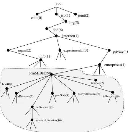
1. PFM MIB: The Pro-active Fault Management (PFM) MIB module defines the objects used to determine the “health” of a UNIX workstation. Figure 1 shows the MIB tree for the PFM module. Note that objects for proprietary MIBs are defined under an organiza-tion’s subtree located under the “enterprises” branch. The module “pfmMIB” is defined asfenterprises 2598gin the MIB tree hierarchy, where the number 2598 is arbitrarily given. The objects to be monitored are classified in the following seven categories, each of which is defined as a placeholder object in the module.

(a) hostID defined as fpfmMIB 1g: The leaf objects in this category, nodeName, osName, osRelease, osVersion and mcHardwareName, characterize the features of the workstation. Since the value of each of these objects is constant, they need to be retrieved by the remote manager/monitor only once.

root

ccitt(0) iso(1) joint(2) org(3)

dod(6)

internet(1)

mgmt(2) experimental(3) _private(4)

enterprises(1)

hostID(1)

osResource(2) procStats(4) fileSysResource(5) timeVal(7)

ioResource(6)

mib(1)

netResource(3)

streamsAllocation(10)

pfmMIB(2598)

Figure 1. MIB tree for the PFM module

(c) osResource defined as fpfmMIB 2g: The leaf objects here describe the state of the re-sources provided by the OS and so some of the objects are operating system dependent. Some of the objects are usedSwapSpace, fileTableSize, realMemoryFree and procsTotal.

(d) procStatsdefined asfpfmMIB 4g: It con-tains leaf objects that describe the state of the processes running on the machine.

(e) fileSysResourcedefined asfpfmMIB 5g: It consists of four leaf objects tmpDirSize, tmpDirUsed, tmpDirAvail and tmpDirCapacity, which keep track of the /tmp directory in UNIX systems.

(f) netResource defined as fpfmMIB 3g: It is a placeholder object in PFM MIB to mon-itor the availability and usage of network re-lated resources provided by the operating sys-tem. Some examples are queuesCurrent, dblksAllocFailandstreamsCurrent.

(g) ioResource is defined as fpfmMIB 6g: It contains information about the terminal as well as disk I/O activity such as ttyIn and diskOneMsps. A total of fourteen leaf objects comprise this category.

2. PFM agent: The agent process runs in the background on each monitored workstation. A single instance for each of the MIB leaf objects is initialized as a global

variable in the agent program. The agent then pas-sively listens on a well advertised port number. Upon receiving agetrequest from the manager, the agent executes certain instructions to obtain the value of the requested leaf object from the operating system, as-signs the value to the variable and sends it back to the manager with the value. This procedure is illustrated in Figure 2. The values for the leaf objects are ob-tained by the agent by executing various UNIX utility programs made available as a standard part of the op-erating system such aspstat,iostat,netstat, vmstat,nfsstat,topanddf.

return (pstat) _value

Operating System Kernel Hardware

Unix Utility return value

(22312K) get(leaf object) (totalSwapSpace)

Agent process

Figure 2. Working of the agent process

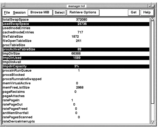
3. PFM Manager: The manager’s primary function is to retrieve the values of desired objects by sendingget requests to the remote agents. We have implemented a graphical user interface which can be operated in one of two modes - “monitoring” and “collection”. While in the monitoring mode, the retrieval of information is initiated by the user (administrator), in the collection mode, it is automated. Figure 3 shows the snapshot of the interface with some selected objects and their associated values.

The prototypes for the agent and the manager programs were developed using Scotty [13]. Scotty is an extension to the Tcl/Tk prototyping language and provides TCP/IP, UDP, ICMP and SNMP functionality. It supports both versions 1 and 2 of SNMP. In our implementation, we have used only SNMP V.1.

4. Data Collection

Figure 3. Snapshot of the GUI for the manager

UNIX workstations which are connected by an Ethernet LAN at the Duke Department of Electrical and Computer Engineering. The machines monitored and their respective operating systems and primary functions in the department are listed in Table 1. In our data collection, the values for all objects are collected every fifteen minutes using the collection mode. The data is stored in a user-specified file in an X-Y format, where X is the name of the object and Y is its value. Any processing on the data is done outside of the tool. In the case of an error or timeout, a “No Response” is recorded. The timeout interval was two minutes. When a monitored machine fails, it is restarted/rebooted and the agent process is also restarted.

5. Data Analysis

Using the monitoring tool, time ordered values are ob-tained for eachpfmMIBobject, thus constituting a time se-ries for that object. In this section, we introduce the time series analysis concepts used to determine the patterns of variation with time in the values of each of the objects. Spe-cific issues we address are:

Is aging present, or in other words, is there a long term trend (increasing or decreasing) in the values?

What is the nature of the variations in values? Does the data exhibit periodic behavior with or without a global/local trend?

Can the failures during this period be related to the ob-served values?

Table 1. Machines monitored at Duke Dept. of ECE

Machine Name Operating System Function

ECE Solaris 2.2 WWW, FTP, mail, NIS, DNS server Washington Solaris 2.3 file server

for programs/packages Lincoln Solaris 2.2 file server for directories,

research printer server Jefferson SunOS 4.1.3 NIS secondary server

Dolphin SunOS 4.1.3 research (usr home directories)

Datc6 Solaris 2.2 public cluster workstation Velum SunOS 4.1.3 research (usr home

directories) Rossby SunOS 4.1.3 research

Shannon AIX research, data collection /monitoring station

Can we quantify aging in UNIX?

To obtain the desired answers, we use visual cues and classical time series analysis techniques such as linear and periodic dependency analysis, and trend detection and estimation [1].

5.1. Time Series Analysis and Time Plots

A time series is simply a set of dataf

y

t

:

t

=1

::: n

gin which the subscript

t

indicates the time at which the datum

y

t is observed. It is a sample realization of a stochastic processf

Y

t

:

t

=1

::: n

g. The expectation of

Y

t, denoted by

t

=

E

Y

t

]is called the trend of the series. In our case, since the observations are made at regular fifteen minute intervals, it suffices to indicate the index of the interval.

Plotting the time seriesf

y

t

:

t

=1

::: n

g against time

forecasting purposes.

5.2. Periodicity and Linear Dependence

To study linear dependency in time, the autocorrelation function is an important, albeit typically incomplete, sum-mary of the serial dependence within a stationary random function. The plot of autocorrelation against lag, called the correlogram of the data, is very useful for exploratory data analysis. In addition to linear dependence, periodic dependencies may be important. To corroborate the presence of periodicities in the data, we employ harmonic analysis, which involves fitting a periodic function of a particular frequency to the data. The existence of daily and weekly periodicities in the measured data can be confirmed via harmonic analysis.

5.3. Trend Detection and Estimation

As mentioned previously, one of the primary objectives of our data analysis is to detect and validate the existence of aging. Detection of trends in operating system resource usage and system activity is the approach we follow. For the purposes of prediction, the slope of the trend is es-timated. The primary trend detection technique used is smoothing of observed data by robust locally weighted re-gression, proposed by Cleveland [4]. The process of ro-bust locally weighted regression essentially involves fitting a polynomial of any desired degree to a fraction of the data. The fitting is carried out using weighted least squares es-timates. The fraction of the data smoothed at each point, called the window size, has a significant effect on the result. A large window size is used to capture the overall trend by removing local variations. With a small window size, the smoothed data points almost follow the original data points. We have used a window size of 2/3 (fraction of all data) for our analysis. The robust smoothing technique provides good visual cues for finding trends in the series

y

t, but it is hard to make conclusive statements regarding presence or absence of trend since no statistical significance levels are attached. To overcome this limitation, we use the seasonal Kendall test [5]. It can be used for detection of trends in the presence of cycles. The duration of a cycle is referred to as the period and the durations within a cycle are called sea-sons. We expect to see daily cycles in our data. The objec-tive in the seasonal Kendall test is to test the null hypothesis

H

0 that there is no trend, against the alternative hypothe-sis

H

A that there is an upward or a downward trend. To that end, we compute for each season

i

the Mann-Kendall

statistic,

S

i, where

S

i =

n i

;1 X

k =1 n

i X

l=k +1

sgn

(

y

il

;

y

ik

) (1)

where

l > k

and

sgn

(

x

) is the signum function,

n

i is the number of data (over cycles) for season i and

y

il is the datum for the

i

th season of the

l

th cycle. To test the null hypothesis,

H

0is rejected for certain values of the

Z

statistic (computed from all the

S

is), for a significance level

(see [5] for details). The seasonal Kendall test is simple, efficient and robust against any missing values in the data.

Once the presence of a trend is confirmed by the above procedure, its true slope may be estimated by computing the least squares estimate of the slope by linear regression methods. These however deviate greatly from the true value if there are gross errors or outliers in the data. We use a non-parametric procedure developed by Sen [18], which is not greatly affected by outliers and is also robust against missing values.

First, for each season

i

,

N

0

i slopes are calculated for all pairs of points at

l

and

k

for which

l > k

as

Q

i = (

y

il ;

y

ik

)

=

(

l

;

k

). These

N

0 1+...+

N

0

K=

N

0 slopes, where

K

is the number of seasons, are then ranked and their median is calculated. This median is the required slope estimate,

N

. A confidence interval can also be attached to the slope.

6. Results

The total time period for our data collection was ap-proximately 53 days. Three machines, Jefferson, Rossby and Velum, did not experience any outage during this period. The other four machines, Dolphin, ECE, Lincoln and Datc6, suffered outages. The number of outages, the time of occurrence of each outage and its probable cause are listed in Table 2. The time of outage is expressed in days:hours:minutes. The probable cause of failure is noted simply by observing the values of the objects just before the failure and identifying resources, if any, that are nearing exhaustion at that time. Failures which did not show any signs of resource exhaustion (presumably due to hardware or other faults) are not considered in our analysis.

Table 2. Observed number, times and proba-ble causes of failures

Machine Outages Time Cause

Dolphin 3 01:21:55 Swap Space Exhausted 20:16:45

50:09:51

ECE 1 16:17:34 Out of Memory Lincoln 4 12:08:03 Out of Memory

30:03:55 Too many messages 38:10:13

45:12:49

Datc6 4 12:08:09 Outages 30:09:47 Correlated 38:11:03 with 45:13:44 Lincoln

Lag

ACF

0 5 10 15 20

0.0

0.4

0.8

Series : Current dblks

Lag

ACF

0 5 10 15 20

-0.2

0.2

0.6

1.0

Series : Current queues

Figure 4. Autocorrelation function for

Jeffer-son objects: (1) current no. of allocated

streams data blocks (2) no. of stream queues

Time (days)

0 10 20 30 40 50

0

2

04

06

0

swapUsed

Time plots for Datc6 objects

Time (days)

0 10 20 30 40 50

0

500

1500

tmpDirUsed

Time (days)

0 10 20 30 40 50

0

40000

80000

tmpDirAvail

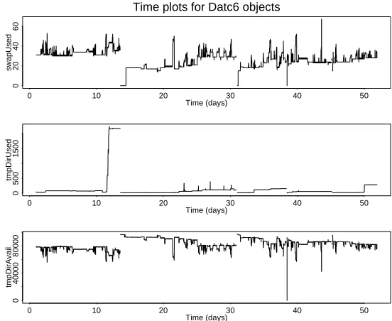
Figure 5. Time plots for Datc6 objects: (1) swap space in use (2) /tmp in use (3) /tmp available

Time (days)

0 10 20 30 40 50

0

400

800

1200

swapUsed

Time plots for ECE objects

Time (days)

0 10 20 30 40 50

0

100000

200000

tmpDirUsed

Time (days)

0 10 20 30 40 50

0

10^6

2*10^6

tmpDirAvail

Time (days)

0 10 20 30 40 50

0

1000

2000

3000

queuesCurrent

Time plots for ECE objects

Time (days)

0 10 20 30 40 50

0

2

04

0

6

08

0

linkblkCurrent

Time (days)

0 10 20 30 40 50

0

2000

6000

msgCurrent

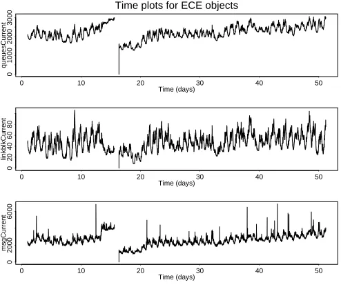
Figure 7. Time plots for ECE objects: (1)

current no. of stream queues (2) linkblk

STREAMS structures allocated (to indicate a link) (3) streams messages allocated

trends. First, we identify linear and periodic dependencies.

Figure 4 shows the autocorrelation functions plotted against lag for two objects monitored in machine Jefferson. Computing the autocorrelation function requires that the time series

y

t be stationary. However, the time series potentially consist of a global trend, which makes them non-stationary. Therefore, this trend,

tis computed using non-parametric regression smoothing and subtracted from the original time series

y

tand the autocorrelation functions are computed for these residual series

y

t

;

tfor lags of up to approximately 20 days. Hence the lag in the plots corresponds to days. Each plot contains two horizontal dashed lines which correspond to 95% confidence limits. Statistically, correlation functions lying inside these bound-aries are considered insignificant.

6.1. Detection of Periodicities and Linear Depen-dence

Figure 4, plots 1 and 2, show significant autocorrelation at the lag which corresponds to a day. As the autocorre-lation persists over all lags (visible as alternating positive and negative peaks), it is a clear indication that the time series has a periodic component with a periodicity of one day. Furthermore, the envelope of the peaks in these plots show that correlations exist at a lag of 7, which corresponds

to a week. This is indicative of the presence of weekly periodicity exhibited by the original time series.

Analysis of periodic dependencies can be done for all objects. Not all objects show daily and weekly dependen-cies as in plots 1 and 2 of Figure 4. Some only show weekly dependencies (for instance caused by periodic maintenance activities), while others show no significant indications of the presence of periodicities or linear dependence.

6.2. Detection and Validation of the Existence of Aging

The existence of aging is some times evident simply from observation of some of the time plots of resources. For instance, a gradual consistent increase in resource usage (disregarding local variations) is visible for some of the ECE objects in Figures 6 and 7. In the case of other resources, however, aging is not evident simply by visual inspection of data. Hence, we resort to the analysis techniques described earlier to detect aging.

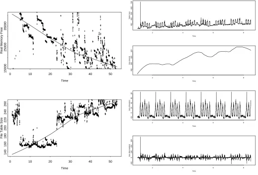
Smoothing of a time series by non-parametric local weighted regression is applied to the time series of objects for Rossby. Figure 8 shows the smoothed data superim-posed on the original data points. Amount of real memory free, plotted in Figure 8, plot 1, shows an overall decrease, whereas process table size shows an increase. We have used the smoothing technique only to get the global trend between outages and so the resulting smoothed data might not always follow the original data points. Plots of some other resources not discussed here also showed an increase or decrease. Once again, this corroborates our hypothesis of aging with respect to various objects.

We also applied the seasonal Kendall test to each of these time series to detect the presence of any global trends at a significance level,

, of 0.05. The associated statistic is listed in Table 3. With

Z

=1.96, all values in the table are such that the

H

0hypothesis (that no trend exists) is rejected.

Time

Real Memory Free

0 10 20 30 40 50

15000

25000

35000

Time

File Table Size

0 10 20 30 40 50

140

160

180

200

220

240

260

Figure 8. Non-parametric regression smooth-ing for Rossby objects: (1) free memory and (2) file table size

Table 3. Seasonal Kendall test (Z Statistic)

for Rossby, Velum and Jefferson objects at

=0.05

Resource Rossby Velum Jefferson

Name

Real Memory Free -13.668 -6.848 -46.977 File Table Size 38.001 17.006 47.065 Process Table Size 40.540 12.142 38.537 Used Swap Space 15.280 32.654 31.660 No. of disk data blocks 48.840 13.955 13.673 No. of queues 39.645 19.906 13.476

Time

Table Size

2 4 6 8

300

400

500

600

700

Time

Size (trend)

2 4 6 8

260

280

300

320

Time

Size (Periodic)

2 4 6 8

-2

0

0

2

04

0

6

08

0

Time

Size (Remainder)

2 4 6 8

-100

0

100

200

300

Figure 9. Trend and seasonal decomposition for Jefferson object file table size against time in weeks

Y

values of the bottom three plots yields the original time series. The difference in scale between the three plots is worth noting as it gives the relative significance of the three components. Particularly noteworthy is the sharp spike present in the original time series as well as the remainder component at around the 2nd day of the first week. This remains unexplained and is attributed to random phenomenon. Such extremely significant yet unexplained transients are present in other time series objects as well.

6.3. Age Quantification and Estimation

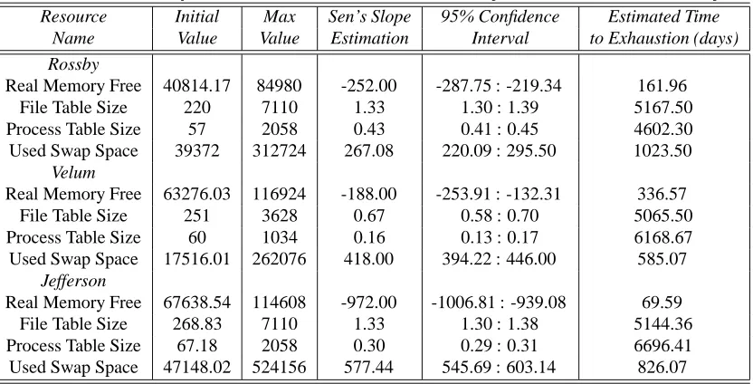
Table 4. Estimated slope and time to exhaustion for Rossby, Velum and Jefferson objects

Resource Initial Max Sen’s Slope 95% Confidence Estimated Time

Name Value Value Estimation Interval to Exhaustion (days)

Rossby

Real Memory Free 40814.17 84980 -252.00 -287.75 : -219.34 161.96 File Table Size 220 7110 1.33 1.30 : 1.39 5167.50 Process Table Size 57 2058 0.43 0.41 : 0.45 4602.30 Used Swap Space 39372 312724 267.08 220.09 : 295.50 1023.50

Velum

Real Memory Free 63276.03 116924 -188.00 -253.91 : -132.31 336.57 File Table Size 251 3628 0.67 0.58 : 0.70 5065.50 Process Table Size 60 1034 0.16 0.13 : 0.17 6168.67 Used Swap Space 17516.01 262076 418.00 394.22 : 446.00 585.07

Jefferson

Real Memory Free 67638.54 114608 -972.00 -1006.81 : -939.08 69.59 File Table Size 268.83 7110 1.33 1.30 : 1.38 5144.36 Process Table Size 67.18 2058 0.30 0.29 : 0.31 6696.41 Used Swap Space 47148.02 524156 577.44 545.69 : 603.14 826.07

aging only. Table 4 refers to several objects on Rossby, Velum and Jefferson and lists an estimate of the slope (change per day) of the trend obtained by applying Sen’s non-parametric method. The values for real memory and swap space are in Kilobytes. A negative slope, as in the case of real memory, indicates a decreasing trend, whereas a positive slope, as in the case of file table size, is indicative of an increasing trend. Given the slope estimate, the table lists the estimated time to failure of the machine due to aging only with respect to this particular resource. The calculation of the time to exhaustion is done by using the initial intercept,

c

, the calculated slope,

m

, and a standard linear approximation

y

=

mx

+

c

. The value of the intercept

c

is taken to be the mean of the ini-tial 5 days. The minimum value for all the resources is zero.

A comparative effect of aging on different system resources can be obtained from the above estimates. For example, in machine Rossby, the resource used swap space has the highest slope and real memory free has the second highest slope. Therefore, used swap space has the highest rate of exhaustion. However, when we compare the estimated times to exhaustion of both these resources, real memory free has a gives a lower time to exhaustion than used swap space. This is because of the difference in the initial and maximum/minimum values of these resources. Similar comparisons of slope and estimated time to exhaustion can be done on other machines. Overall, we find that the two resources file table size and process table size are not as important as used swap space and real memory free since they have

a very small slope and high estimated times to failure due to exhaustion. Based on such comparisons, we can identify important and interesting resources to moni-tor and manage, to deal with aging related software failures.

The estimated time to resource exhaustion can be taken to be the estimated time of failure of the machine due to that particular resource. It is important to note that this only considers failure due to aging of a particular resource alone. For a more general failure prediction, the occurrence of transients in resource usage, as well as the combined effect of aging, periodic component and transient component, need to be modeled and understood. Additionally, the interaction and correlation between the usage of various resources and their impact on system availability remains to be explored. It is precisely for these reasons that the estimated times of failures done this way do not fully explain the actual times of failure observed on various machines. The estimated time to resource exhaustion and slope however can be used to study the aging phenomena which is a very important element in software failures. Prediction methods based on aging become important, especially in light of fault-tolerance techniques such as software rejuvenation where the time of actual rejuvenation is an issue.

7. Conclusion

Based on SNMP, the tool is inter-operable among machines running UNIX and its variants. We also described the data collection process accomplished via monitoring operating system resource usage and system activity. The primary contribution of our work is a methodology for detecting and estimating aging in operational software. Based on this, we proposed a metric, “Estimated time to exhaustion”, for each resource as a quantification of aging. The higher this metric is, lower is the effect of aging on this resource. This metric helps in comparing the effect of aging on different system resources and also in the identification of important resources to monitor and manage. This is also a first step towards predicting aging related failure occurrences, and may help us in developing a strategy for software fault-tolerance approaches, such as software rejuvenation, triggered by actual measurements.

References

[1] G. E. P. Box, G. M. Jenkins, and G. C. Reinsel. Time Series Analysis: Forecasting and Control. Prentice Hall, Englewood Cliffs, NJ, 1994.

[2] J.D. Case, M. Fedor, M.L. Schoffstall, C. Davin, M. T. Rose, and K. McCloghrie. Simple Network Management Protocol. RFC 1157, May 1990.

[3] R. Chillarege, S. Biyani, and J. Rosenthal. Measurement of failure rate in widely distributed software. In Proc. of 25th IEEE Intl. Symposium on Fault-Tolerant Computing, pages 424-433, Pasadena, CA, July 1995.

[4] W. S. Cleveland. Robust locally weighted regression and smoothing scatterplots. Journal of the American Statistical Association, 74(368):829-836, December 1979.

[5] R. O. Gilbert. Statistical Methods for Environmental Pollution Monitoring. Van Nostrand Reinhold, New York, NY, 1987. [6] J. Gray and D. P. Siewiorek. High-availability computer

sys-tems. IEEE Computer, pages 39-48, September 1991. [7] J.P. Hansen and D.P. Siewiorek. Models for time coalescence

in event logs. In Proc. of 22nd IEEE Intl. Symposium on Fault-Tolerant Computing, pages 221-227, 1992.

[8] Y. Huang, P. Jalote, and C. Kintala. Lecture Notes in Com-puter Science, Vol. 774, Two techniques for transient software error recovery, pages 159-170. Springer Verlag, Berlin, 1994. [9] Y. Huang, C. Kintala, N. Kolettis, and N. D. Fulton. Software rejuvenation: Analysis, module and applications. In Proc. of 25th IEEE Intl. Symposium on Fault-Tolerant Computing, pages 381-390, Pasadena, California, June 1995.

[10] R.K. Iyer and D.J. Rossetti. Effect of system workload on op-erating system reliability: a study on IBM 3081. IEEE Trans-actions on Software Engineering, SE-11(12):1438-1448, Dec. 1985.

[11] R. K. Iyer, L. T. Young, and P. V. K. Iyer. Automatic recog-nition of intermittent failures: An experimental study of field data. IEEE Transactions on Computers, 39(4):525-537, April 1990.

[12] P. Jalote, Y. Huang, and C. Kintala. A framework for under-standing and handling transient software failures. In Proc. of 2nd ISSAT Intl. Conf. on Reliability and Quality in Design, Orlando, Florida, 1995.

[13] H. Langendorfer J. Schonwalder. Tcl extensions for network management applications. In Proc. of 3rd Tcl/Tk Workshop, Toronto (Canada), July 1995.

[14] I. Lee, R. K. Iyer, and A. Mehta. Identifying software prob-lems using symptoms. In Proc. of 24th IEEE Intl. Symposium on Fault-Tolerant Computing, Toulouse, France, June 1994. [15] T-T. Lin and D. P. Siewiorek. Error log analysis: Statistical

modeling and heuristic trend analysis. IEEE Transactions on Reliability, 39(4):419-432, October 1990.

[16] R. A. Maxion and F. E. Feather. A case study of Ether-net anomalies in a distributed computing environment. IEEE Transactions on Reliability, 39(4), 1990.

[17] M. T. Rose and K. McCloghrie. Structure and Identifica-tion of Management InformaIdentifica-tion for TCP/IP-based Internets. RFC 1155, May 1990.

[18] P. K. Sen. Estimates of the regression coefficient based on Kendall’s tau. Journal of the American Statistical Associa-tion, 63:1379-1389, 1968.

[19] M. Sullivan and R. Chillarege. Software defects and their impact on system availability - a study of field failures in op-erating systems. In Proc. of 21st IEEE Intl. Symposium on Fault-Tolerant Computing, pages 2-9, 1991.

[20] D. Tang and R. K. Iyer. Dependability measurement model-ing of a multicomputer system. IEEE Transactions on Com-puters, 42(1), January 1993.