A Survey on the Performance Analysis of WT,
PF, EMD & EEMD Methods used in ECG
Signal Processing
Mohit Tyagi 1, Ranjeeta Yadav 2
P. G. Student, Department of Electronics & Communication Engineering, ABES Engineering College, Ghaziabad, Uttar Pradesh, India 1
Sr. Assistant Professor, Department of Electronics & Communication Engineering, ABES Engineering College, Ghaziabad, Uttar Pradesh, India 1
ABSTRACT: A noiseless ECG identification technology is an emerging new biometric modality. Different
techniques for de-noising of ECG signal are prevalent in recent literatures such as Particle Filter (PF), wavelet transforms (WT), Empirical Mode Decomposition (EMD) & Ensemble-EMD Method. In view of the fact that Analysis of ECG signals becomes difficult to inspect the cardiac activity in the presence of Noise signals. So, de-noising of ECG signal is extremely important to prevent misinterpretation of patient’s cardiac activity which can lead to wrong diagnosis and further to death. This paper is surveying a comparison on the performance of the Particle Filter (PF), wavelet transforms (WT) and Empirical Mode Decomposition (EMD) & Ensemble EMD methods in context of de-noising of an electrocardiogram (ECG) signal. Analysis of the paper provides us the way of selecting best de-de-noising technique of ECG signal based on the numerical value in terms of SNR and RMSE. The study is limited to signals corrupted by additive white Gaussian random noise.
KEYWORDS: Empirical mode decomposition (EMD), intrinsic mode function (IMF), Particle filter, Wavelet
transform, Hilbert–Huang transform (HHT), SNR, RMSE.
1. INTRODUCTION
Fig. 1Normal ECG Waveform
The amplitude and duration of the P-Q-R-S-T-U wave more specifically QRS complex contains the first hand example of electrocardiogram waveform which consists of a P, QRS, T and small U wave is noticeable in certain cases. In the regular heartbeat, the key parameters are examined which comprise the duration, shape, R-R interval and QRS complex wave of electrocardiogram signal as whole. The fluctuation in these parameters leads to illness of the heart. ECG picks up electrical impulses generated by the polarization and depolarization of cardiac tissue and translates into a waveform. Normal rhythm produces four entities as shawn below in figure.1 — a P wave, a QRS complex, a T wave, and a U wave — that each have a fairly unique pattern.
The P wave represents a trial depolarization.
The QRS complex represents ventricular depolarization.
The T wave represents ventricular repolarization.
The U wave represents papillary muscle repolarization.
ECG signal is contaminated with various artifacts during acquisition for example Power line interference(PLI), Patient electrode motion artifacts, Electrode-pop or contact noise, and Baseline Wandering and Electromyographic (EMG) noise. Analysis of ECG signals becomes difficult to inspect the cardiac activity in the presence of such unwanted signals. So, de-noising of ECG signal is extremely important to prevent misinterpretation of patient’s cardiac activity. The paper is organized in such a way that Section II provides the related work, section III provides the theoretical analysis of denoising techniques such as WT, PF, EMD & EEMD algorithm. Section IV provides the results making a comparison of Four different techniques for de-noising of ECG signal. Finally the conclusion is drawn in this section V.
II. RELATED WORK
used HHT to analyze satellite scatterometer wind data over the northwestern Pacific and compared the results to vector empirical orthogonal function (VEOF) results. Schlurmann [2002] introduced the application of HHT to characterize nonlinear water waves from two different perspectives, using laboratory experiments. Veltcheva [2002] applied HHT to wave data from nearshore sea. Larsen et al. [2004] used HHT to characterize the underwater electromagnetic environmentand identify transient manmade electromagnetic disturbances. Huang et al. [2001] used HHT to develop a spectral representation of earthquake data. Chen et al. [2002] used HHT to determined the dispersion curves of seismic surface waves and compared their results to Fourier-based time-frequency analysis. Shen et al. [2003] applied HHT to ground motion and compared the HHT result with the Fourier spectrum. Nakariakov et al. [2010] used EMD to demonstrate the triangular shape of quasi-periodic pulsations detected in the hard X-ray and microwave emission generated in solar flares. Barnhart and Eichinger [2010] used HHT to extract the periodic components within sunspot data, including the 11-year Schwabe, 22-year Hale, and ~100-year Gleissberg cycles. They compared their results with traditional Fourier analysis. Quek et al. [2003] illustrate the feasibility of the HHT as a signal processing tool for locating an anomaly in the form of a crack, delamination, or stiffness loss in beams and plates based on physically acquired propagating wave signals. Using HHT, Li et al. [2003] analyzed the results of a
pseudodynamic test of two rectangular reinforced concrete bridge columns. Pines and Salvino [2002] applied HHT in structural health monitoring. Yang et al. [2004] used HHT for damage detection, applying EMD to extract damage spikes due to sudden changes in structural stiffness. Yu et al. [2003] used HHT for fault diagnosis of roller bearings. Parey and Pachori (2012) have applied EMD for gear fault diagnosis. Chen and Xu [2002] explored the possibility of using HHT to identify the modal damping ratios of a structure with closely spaced modal frequencies and compared their results to FFT. Xu et al. [2003] compared the modal frequencies and damping ratios in various time increments and different winds for one of the tallest composite buildings in the world. Huang and Pan [2006] have used the HHT for speech pitch determination.
III. THEORETICAL ANALYSIS
A brief description of various techniques such as EMD, Wavelet transform and Particle Filter used for de-noising of ECG signal in this section. Hilbert-Huang Transform (HHT) was presented by Huang et.al [2], is the combination of Hilbert Transform and EMD. It is very much appropriate for non-stationary and nonlinear signal processing. This transform presents two phases for signal processing. First, Original dataset is converted into an ‘n’ (number of) Intrinsic Mode Functions (IMFs) through EMD method and then these IMFs components are passed through Hilbert Transform.
This section also shows that the limitation of EMD is overcomed through using EEMD method.
A. WAVELET TRANSFORM
Wavelet transform is a multi-resolution study as developed by Mallat [5].The wavelet transform evaluates signals in both time and frequency domains unlike Fourier Transform. It is widely used for the non-stationary signals. The wavelet transform was developed to overcome the limitations of STFT. The Wavelet Transform can be classified into continuous and discrete.
Continuous wavelet transforms (CWT) [5] :The Continuous wavelet transform represents a signal as a function of time and scale. The CWT is obtained by changing the scale of the analysis window, shifting the window in time, multiplying the signal and integrating the result over all time.
The CWT of a f (t) is given by
f(t) = ∬∞, ∞ ( , ) , ( ) (1)
W(a,b) = ∫∞∞ ( )
√І Іψ *
Where a is the scaling parameter and b is shifting parameter. Both a and b are real in nature. The scale parameter ‘a’ gives the frequency information whereas translation parameter ‘b’ gives the time information.
The Inverse CWT is given by
C = ∫∞∞| ( )|| | d (3)
Discrete wavelet transform (DWT): The discrete WT is obtained by filtering the signal through a series of digital filters at different scales. The DWT of a signal is calculated by passing it through a series of filters. First the samples are passed through a low-pass filter with impulse response which gives the convolution of two signals. Due to the rate-change operators in the filter bank, the discrete WT is not time-invariant but actually very sensitive to the alignment of the signal in time. To address the time-varying problem of wavelet transforms, Mallat and Zhong proposed a new algorithm for wavelet representation of a signal, which is invariant to time shifts. According to this algorithm, which is called a TI-DWT, only the scale parameter is sampled along the dyadic sequence and the wavelet transform is calculated for each point in time.
B. PARTICLE FILTER [7]
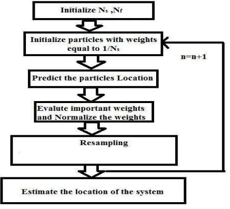
PF is a Bayes estimation algorithm based on Monte Carlo method. It performs the posterior probability density function via a number of weighted particles and eliminates particles that have small weights and concentrates on particles with large weights using resample. A common problem with the SIS particle filter is the degeneracy phenomenon, where after a few iterations; all but one particle will have negligible weight. When using a particle filter, one can often expect and frequently achieve an improvement in performance by using far more particles or alternatively by employing regularization or using an auxiliary particle filter.
Fig. 2 Particle Filter
P "particles" at k using only the particles from (k-1). This requires that a Markov equation can be written (and computed) to generate a ( Xk ) based only upon ( Xk-1 ). This algorithm uses composition of the P particles from (k-1) to generate a particle at k and repeats Process until P particles are generated at k.
C. EMPIRICAL MODE DECOMPOSITION (EMD)
The Hilbert–Huang transform (HHT) is designed to work well for data that is nonstationary and nonlinear. In contrast to other common transforms like the Fourier transform, the HHT is more like an algorithm (an empirical approach) that can be applied to a data set, rather than a theoretical tool. The Hilbert–Huang transform (HHT) was proposed by Huang et al. a NASA designated. It is the combination of the empirical mode decomposition (EMD) and the Hilbert spectral analysis (HSA). The HHT uses the Empirical mode decomposition, an iterative process to decompose real signals into so-called intrinsic mode functions (IMF) with a trend, and applies the HSA method to the IMFs to obtain instantaneous frequency data. Since the signal is decomposed in time domain and the length of the IMFs is the same as the original signal, HHT preserves the characteristics of the varying frequency. This is an important advantage of HHT since real-world signal usually has multiple causes happening in different time intervals. Infact HHT provides a new method of analyzing nonstationary and nonlinear time series data.
Empirical mode decomposition (EMD) is the fundamental part of the HHT i.e an iterative process of Breaking down signals into various component, EMD can be compared with other analysis method such as Fourier transform, Wavelet transform & Particle Filter. Using the EMD Algorithm technique, any complicated data set can be decomposed into a finite and often small number of components. These components form a complete and nearly orthogonal basis for the original signal. In addition, they are described as intrinsic mode functions (IMF). Even in the time domain EMD is adaptive and highly efficient.
The starting point of the Empirical Mode Decomposition (EMD) is to consider signals at the level of their local oscillations. Looking at the evolution of a signal x(t) between two consecutive local extrema (say, two minima occurring at times t− and t+), we can heuristically define a (local) high frequency part {d(t), t− ≤ t ≤ t+}. Also called detail, d(t)corresponds to the oscillation terminating at the two minima and passing through the maximum which necessarily exists in between them.
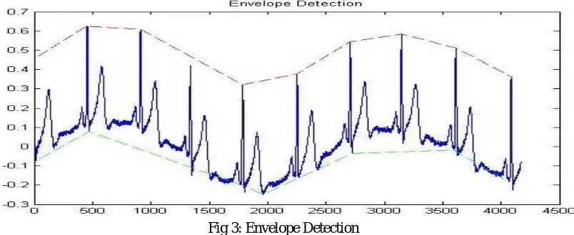
Given a signal x(t), the effective algorithm of EMD can be summarized as follows [11]: 1. identify all extrema of x(t)
2. interpolate between minima (resp. maxima), ending up with some “envelope” emin(t) (resp. emax(t))
3. compute the average m(t) = (emin(t) + emax(t))/2
4. extract the detail d(t) = x(t) − m(t)
5. iterate on the residual m(t)
Fig 3: Envelope Detection
detail signal d(t), until this latter can be considered as zero-mean according to some stopping
criterion. Once this is achieved, the detail is considered as the effective IMF, the corresponding residual is computed and step 5 applies. By construction, the number of extrema is decreased when going from one residual to the next (thus guaranteeing that the complete decomposition is achieved in a finite number of steps), and the corresponding spectral supports are expected to decrease accordingly.
While modes and residuals can intuitively be given a “spectral” interpretation, it is worth stressing the fact that, in the general case, their high vs. low frequency discrimination applies only locally and corresponds by no way to a pre-determined sub-band filtering (as, e.g., in a wavelet transform). Selection of modes rather corresponds to an automatic and adaptive (signal-dependent) time-variant filtering.
The major disadvantage of EMD is the mode mixing consequence. And the End effect as well as unstablity is also a problem with EMD. Mode-mixing shows that the oscillations of different time scales co-exist in a given IMF or oscillations with the similar time scale is being allocated to different IMFs. In 2D versionthe main disadvantage of EMD is the decomposition in two dimensions is extremely time consuming.
D. ENSEMBLE-EMD
EEMD utilizes the scale separation capability of the EMD, and enables the EMD method to be a truly dyadic filter bank for any data. By adding finite noise, the EEMD eliminated largely the mode mixing problem and preserve physical uniqueness of decomposition. Therefore, the EEMD represents a major improvement of the EMD method.
The basic principle of the EEMD is to separate signals of different scales without undue mode mixing. Adding white noise helps to establish a dyadic reference frame in the time–frequency or timescale space. The real data with a comparable scale can find a natural location to reside.
The EEMD utilizes all the statistical characteristic of the noise: it helps to perturb the signal and enable the EMD algorithm to visit all possible solutions in the finite (not infinitesimal) neighborhood of the true final answer; it also takes advantage of the zero mean of the noise to cancel out this noise background once it has served its function of providing the uniformly distributed frame of scales, a feat only possible in the time-domain data analysis.
Mode Mixing Problem: “Mode mixing” is defined as any IMF consisting of oscillations of dramatically disparate scales, often caused by intermittency of the driving mechanisms. When mode mixing occurs, an IMF can cease to have physical meaning by itself, suggesting falsely that there may be different physical processes represented in a mode. Even though the final time–frequency projection could rectify the mixed mode to some degree, the alias at each transition from one scale to another would irrecoverably damage the clean separation of scales. Such a drawback was first illustrated by Huang et al.2 in which the modeled data was a mixture of intermittent highfrequency oscillations riding on a continuous low-frequency sinusoidal signal. An almost identical example used by Huang et al.2 is presented here in detail as an illustration[7].
End effect: End effect occurs at the beginning and end of the signal because there is no point before the first data point and after the last data point to be considered together. In most cases, these end points are not the extreme value of the signal. While doing the EMD process of the HHT, the extreme envelope will diverge at the end points and cause significant error. This error distorts the IMF waveform at its endpoints. Furthermore, the error in the decomposition result accumulates through each repetition of the sifting process[10].
EEMD can be summarized as follows [12]: 1. Add a white noise series to the targeted data.
2. Decompose the data with added white noise into IMFs.
3. Repeat step 1 and step 2 again and again, but with different white noise series each time. 4. Obtain the (ensemble) means of corresponding IMFs of the decompositions as the final result.
The effects of the decomposition using the EEMD are that the added white noise series cancel each other in the final mean of the corresponding IMFs; the mean IMFs stay within the natural dyadic filter windows and thus significantly reduce the chance of mode mixing and preserve the dyadic property.
Intrinsic Mode Functions (IMF): An IMF is defined as a function ψ of a real variable t then it must satisfy the following
two conditions.
Ψhas exactly one zero between any two consecutive local extrema..
ψ has zero “local mean.”
IV. PERFORMANCE EVALUTION MEASURES
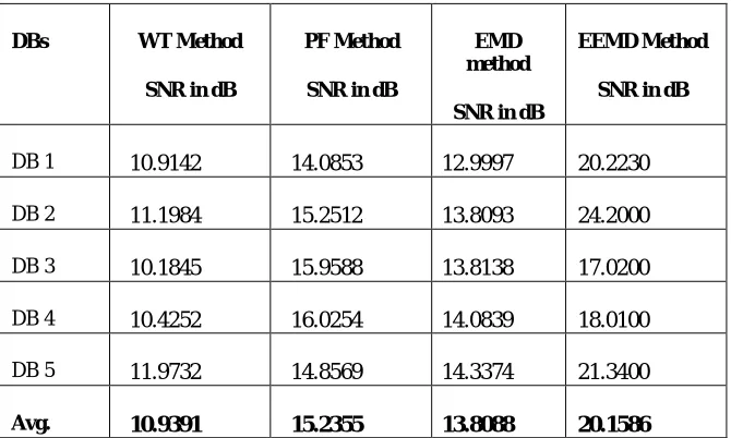
The performance of PF, WT and EMD Algorithms in De-noising of ECG Signal is estimated based on the SNR and RMSE. SNR and RMSE stands for Signal to Noise Ratio and Root Mean square Error respectively. These parameters are used to compare a various existing method. A comparasion of Wavelet Transform, Particle Filter, EMD & Ensemble EMD in terms of SNR & RMSE (Values are given in dB) is shawn in table below[10]. Each method is applied for defferent databases and the values of SNR and RMSE are recorded to compare them further.
Table 4.1 SNR COMPARISON
On camparing table 4.1 it is very clear that average SNR (dB) for EEMD method in four existing methods is superior to all and it is also an empirical approach. As the disadvantages in EMD is overcame in EEMD algorithm so EEMD method is superiour to WT, PF & EMD in veiw of the fact that EEMD shows good SNR results.
DBs WT Method
SNR in dB
PF Method
SNR in dB
EMD method
SNR in dB
EEMD Method
SNR in dB
DB 1 10.9142 14.0853 12.9997 20.2230
DB 2 11.1984 15.2512 13.8093 24.2000
DB 3 10.1845 15.9588 13.8138 17.0200
DB 4 10.4252 16.0254 14.0839 18.0100
DB 5 11.9732 14.8569 14.3374 21.3400
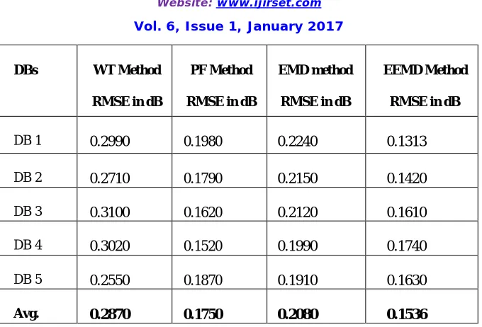
Table 4.2 RMSE COMPARISON
On comparing tables 4.1 & 4.2, it is very clear that the performance of the Ensemble Empirical Mode Decomposition (EEMD) algorithm is better than the existing algorithms with different types of artifacts. The SNR results of the EEMD algorithm show better results and lower Root Mean square Error (RMSE) compared to EMD, Wavelet & PF methods. In view of the fact that mode mixing problem is also reduced in the EEMD method so in that sense this process of decomposition of signal & reconstruction to denoise the ecg signal is superiour to all these methods.
V. CONCLUSION
Many investigator were introduced the various approaches and methods for ECG signal processing or to de-noise them. This paper provides us a comparison between EEMD, EMD, Wavelet and particle algorithms. This paper includes applicability of such methods to ECG de-noising, their advantages and disadvantages. The comparative analysis of different methods presented reveal that the Particle filtering is more efficient than the Wavelet and EMD de-noising method, but EEMD is superior to all, in terms of the signal-to-noise ratio and Root mean square error to improve corrupted ECG signals. The analysis of the paper provides us the way of selection of the best de-noising technique of ECG signal based on the iterative process of decomposing signal as described in EEMD algorithm.
REFERENCES
[1] Neeraj kumar, Imteyaz Ahmad, Pankaj Rai “Signal processing of ECG using Matlab” International journal of Scientific and Reasearch Publications, volume 2,Issue 10, October 2012 pg no.1-6.
[2] N.E. Huang, Z. Shen, S.R. Long, M.L. Wu, H.H. Shih, Q. Zheng, N.C. Yen, C.C. Tung and H.H. Liu, “The empirical mode decomposition and Hilbert spectrum for nonlinear and non-stationary time series analysis,” Proc. Roy. Soc. London A, Vol. 454, pp. 903– 995, 1998.
[3] Changnian Zhang, XiaLi and Mengmeng Zhang, “A novel ECG signal denoising method based on Hilbert-Huang Transform” International Conference on Computer and Communication Technologies in Agriculture Engineering 2010.
[4] Anil Chacko and Samit Ari, “Denoising of ECG signals Decomposition” IEEE International Conference On using Empirical Mode based technique Advances In Engineering, Science And Management (lCAESM -2012) March 30, 31, 2012.
[5] A Wavelet Tour of Signal Processing, 3rd ed. Stéphane Mallat. Academic Press, dec . 2008.
[6] Digital Image Processing, S. Jayaraman, S. Esakkirajan And T. Veerakumar. Tata McGraw - Hill Education Pvt. Ltd.
[7] M. Arulampalam, S. Maskell, N. Gordon and T. Clapp, “A turorial on particle filters for online nonlinear/non-Gaussian Bayesian tracking,”IEEE Trans. On Signal Proc. 50 (2), pp. 174-188, 2002.
[8] P. Flandrin and P. Gonçalves, “Empirical mode decompositions as data-driven wavelet-like expansions,” Int. J. Wavelets, Multires., Inf. Process., vol. 2, no. 4, pp. 477–496, 2004.
DBs WT Method
RMSE in dB
PF Method
RMSE in dB
EMD method
RMSE in dB
EEMD Method
RMSE in dB
DB 1 0.2990 0.1980 0.2240 0.1313
DB 2 0.2710 0.1790 0.2150 0.1420
DB 3 0.3100 0.1620 0.2120 0.1610
DB 4 0.3020 0.1520 0.1990 0.1740
DB 5 0.2550 0.1870 0.1910 0.1630
[9] Fakroul Ridzuan Hashim, Lykourgos Petropoulakis, John Soraghan and Sairul Izwan Safie ,“ Wavelet Based Motion Artifact Removal for ECG Signals”, 2012 IEEE EMBS International Conference on Biomedical Engineering and Sciences I Langkawi I 17th - 19th December 2012. [10] Sarang L. Joshi, Rambabu A. Vatti and Rupali V.Tornekar,“ A Survey on ECG Signal De-noising Techniques”, 2013 International Conference
on Communication Systems and Network Technologies,IEEE 2013.
[11] George Tsolis and Thomas D. Xenos, “Signal Denoising Using Empirical Mode Decomposition and Higher Order Statistics” International Journal of Signal Processing, Image Processing and Pattern Recognition Vol. 4, No. 2, June, 2011.