Analysis of the Sign Regressor Least Mean Fourth Adaptive Algorithm

(1)

Volume 2011, Article ID 373205,12pages doi:10.1155/2011/373205

Research Article

Analysis of the Sign Regressor Least Mean Fourth

Adaptive Algorithm

Mohammed Mujahid Ulla Faiz, Azzedine Zerguine (EURASIP Member),

and Abdelmalek Zidouri

Electrical Engineering Department, King Fahd University of Petroleum and Minerals, Dhahran 31261, Saudi Arabia

Correspondence should be addressed to Azzedine Zerguine,[email protected] Received 25 June 2010; Accepted 5 January 2011

Academic Editor: Stephen Marshall

Copyright © 2011 Mohammed Mujahid Ulla Faiz et al. This is an open access article distributed under the Creative Commons Attribution License, which permits unrestricted use, distribution, and reproduction in any medium, provided the original work is properly cited.

A novel algorithm, called the signed regressor least mean fourth (SRLMF) adaptive algorithm, that reduces the computational cost and complexity while maintaining good performance is presented. Expressions are derived for the steady-state excess-mean-square error (EMSE) of the SRLMF algorithm in a stationary environment. A suﬃcient condition for the convergence in the mean of the SRLMF algorithm is derived. Also, expressions are obtained for the tracking EMSE of the SRLMF algorithm in a nonstationary environment, and consequently an optimum value of the step-size is obtained. Moreover, the weighted variance relation has been extended in order to derive expressions for the mean-square error (MSE) and the mean-square deviation (MSD) of the proposed algorithm during the transient phase. Computer simulations are carried out to corroborate the theoretical findings. It is shown that there is a good match between the theoretical and simulated results. It is also shown that the SRLMF algorithm has no performance degradation when compared with the least mean fourth (LMF) algorithm. The results in this study emphasize the usefulness of this algorithm in applications requiring reduced implementation costs for which the LMF algorithm is too complex.

1. Introduction

Reduction in complexity of the least mean square (LMS) algorithm has always received attention in the area of adaptive filtering [1–3]. This reduction is usually done by clipping either the estimation error or the input data, or both to reduce the number of multiplications necessary at each algorithm iteration. The algorithm based on clipping of the estimation error is known as the sign error or more commonly the sign algorithm (SA) [4–8], the algorithm based on clipping of the input data is known as the sign regressor algorithm (SRA) [9–12], and the algorithm based on clipping of both the estimation error and the input data is known as the sign sign algorithm (SSA) [13,14]. These algorithms result in a performance loss when compared with the conventional LMS algorithm [9, 10]. However, significant reduction in computational cost and simplified hardware implementation can justify this poor performance in applications requiring reduced implementation costs [15,

16].

The behavior of the SRA algorithm depends on the input data. It is shown in [11] that for some inputs, the LMS algorithm is stable while the SRA algorithm is unstable. This is a drawback of the SRA algorithm when compared with the SA algorithm since the latter is more stable than the LMS algorithm [4,16]. The SRA algorithm is always stable when the input data is Gaussian as in the case of speech processing. Also, the performance of the SRA algorithm is superior to that of the SA algorithm for Gaussian input data. It is shown in [10] that the SRA algorithm is much faster than the SA algorithm in achieving the desired steady-state mean-square error for white Gaussian data. Theoretical studies of the SRA algorithm with correlated Gaussian data in both stationary and nonstationary environments are found in [12].

(2)

by a factor of 2/π for the same steady-state mean-square error.

It is shown in [17] that the SRA algorithm exhibits significantly higher robustness against the impulse noise than the LMS algorithm.

The above-mentioned advantages motivate us to analyze the proposed sign regressor least mean fourth (SRLMF) adaptive algorithm. In this paper, the mean-square analysis, the convergence analysis, the tracking analysis, and the transient analysis of the SRLMF algorithm are carried out. The framework used in this work relies on energy conservation arguments [18]. Expressions are evaluated for the steady-state excess-mean-square error (EMSE) of the SRLMF algorithm in a stationary environment. A condition for the convergence of the mean behavior of the SRLMF algorithm is also derived. Also, expressions for the tracking EMSE in a nonstationary environment are presented. An optimum value of the step-sizeμis also evaluated. Moreover, an extension of the weighted variance relation is provided in order to derive expressions for the mean-square error (MSE) and the mean-square deviation (MSD) of the proposed algorithm during the transient phase. From the simulation results it is shown that both the SRLMF algorithm and the least mean fourth (LMF) algorithm [19] have a similar performance for the same steady-state EMSE. Moreover, the results show that the theoretical and simulated results are in good agreement.

The paper is organized as follows: following the Intro-duction is Section 2 where the proposed algorithm is developed, while the mean-square analysis of the proposed SRLMF algorithm is presented inSection 3. The convergence analysis of the proposed algorithm is presented inSection 4.

Section 5presents the tracking analysis of the proposed algo-rithm for random walk channels and as a by-product of this analysis the optimum value of step-size for these channels is derived. AndSection 6presents thoroughly the transient analysis of the proposed algorithm. The Computational Load is detailed inSection 7. To investigate the performance of the proposed algorithm, several simulation results for diﬀerent scenarios are presented inSection 8. Finally, some conclusions are given inSection 9.

2. Algorithm Development

The SRLMF algorithm is based on clipping of the regression vector ui (row vector). Consider now the adaptive filter,

which updates its coeﬃcients according to the following recursion [18]:

wi=wi−1+μH[ui]u∗ig[ei], i≥0, (1)

where wi (column vector) is the updated weight vector at

time i, μ is the step-size, H[ui] is some positive-definite

Hermitian matrix-valued function ofui, g[ei] denotes some

function of the estimation error signal given by

ei=di−uiwi−1, (2)

wheredi is the desired signal. When the data is real-valued

and g[ei]=e3i, the general update form in (1) becomes

wi=wi−1+μH[ui]uTie3i, i≥0. (3)

Now if

H[ui]=diag

1

ui1

,1

ui2

,. . ., 1

uiM

, (4)

then the update form in (3) reduces to

wi=wi−1+μdiag

1

_u_i₁,1

ui2

,. . ., 1

uiM

uT_ie3i

=wi−1+μsign [ui]Te3i, i≥0,

(5)

whereM is the filter length. The SRLMF algorithm update recursion in (5) can be regarded as a special case of the general update form in (3) for some matrix data nonlinearity that is implicitly defined by the following relation:

sign [ui]T=H[ui]uTi. (6)

3. Mean-Square Analysis of

the SRLMF Algorithm

We wil assume that the data {di,ui} satisfy the following

conditions of the stationary data model [18,20–24].

(A.1) There exists an optimal weight vectorwo _{such that} di=uiwo+vi.

(A.2) The noise sequenceviis independent and identically

distributed (i.i.d.) with varianceσ2

v =E[|vi|2] and is

independent ofu_jfor alli,j.

(A.3) The initial conditionw−1is independent of the zero

mean random variables{di,ui,vi}.

(A.4) The regressor covariance matrix isR=E[u∗_iui]>0.

For any adaptive filter of the form in (1), and for any data{di,ui}, assuming filter operation in steady-state, the

following variance relation holds [18]:

μEui2Hg2[ei]

=2Eeaig[ei]

, asi−→ ∞, (7) where

Eui2H

=EuiH[ui]uTi

, (8)

ei=eai+vi, (9)

andeai=ui(wo−wi−1) is the a priori estimation error. Then

g[ei] becomes

g[ei]=ei3= eai+vi

e2

ai+v

2

i + 2eaivi

. (10) By using the fact thateai andviare independent, we reach at

the following expression for the term E[eaig[ei]]:

Eeaig[ei]

=3σ2

vE

e2

ai

+ Ee4

ai

(3)

Ignoring third and higher-order terms of eai, then (11)

becomes

Eeaig[ei]

≈3σ2

vE

e2

ai

. (12)

To evaluate the term E[ui2Hg2[ei]], we start by noting that

g2[ei]=e6ai+ 6e

5

aivi+ 6eaiv

5

i + 15e4aiv

2

i + 15e2aiv

4

i

+ 20e3

aiv

3

i +v6i.

(13)

If we multiply g2_[_e

i] byui2Hfrom the left, use the fact that

viis independent of bothuiandeai, and again ignoring third

and higher-order terms ofeai, we obtain

Eui2Hg2[ei]

≈6Eui2Heaiv

5

i

+ 15Eui2He2aiv

4

i

+ Eui2Hv6i

≈6Eui2Heai

Ev5

i

+ 15Eui2He2ai

×Ev4

i

+ Eui2H

Evi6

≈6Eui2Heai

Ev5

i

+ 15Eui2He2ai

ξ4

v

+ Eui2H

ξ6

v,

(14)

where ξ4

v = E[|vi|4], ξv6 = E[|vi|6] denote the forth and

sixth-order moments ofvi, respectively.

From Price’s theorem [25] we have

Exsign y=

2

π

1

σy

Exy, (15)

then

Eu_i2 H

=Eu_isign [u_i]T=

2

πσ2

u

Tr(R). (16)

Substituting (16) into (14) we get

Eui2Hg2[ei]

≈6Eui2Heai

Ev5

i

+ 15Eui2He2ai

ξ4

v

+

2

πσ2

u

Tr(R)ξv6.

(17)

Substituting (12) and (17) into (7) we get

6σ2

vE

e2

ai

=μξ6

v

2

πσ2

u

Tr(R) + 15μξ4

vE

ui2He2ai

+ 6μEui2Heai

Evi5

.

(18)

In order to simplify (18) and arrive at an expression for the steady-state EMSEζ=E[e2

ai], we consider two cases.

(1) Suﬃciently Small Step-Sizes. Small step-sizes lead to small values of E[e2

ai] andeai in steady-state. Therefore, for

smaller values ofμ, the last two terms in (18) can be ignored, the steady-state EMSE is given by

ζ= μξv6

6σ2

v

2

πσ2

u

Tr(R). (19)

(2) Separation Principle. For larger values of μ, we resort to the separation assumption, namely, that at steady-state,

ui2His independent ofeai. In this case, the last term in (18)

will be zero sinceeaiis zero mean, the steady-state EMSE can

be shown to be

ζ= μξ

6

v

2/πσ2

uTr(R)

6σ2

v−15μξv4

2/πσ2

uTr(R)

. (20)

4. Convergence Analysis of

the SRLMF Algorithm

Convergence analysis of the SRLMF algorithm is much more complicated than that of the LMS algorithm due to existence of the higher order estimation error signal in the coeﬃcient update recursion. We thus make the following assumptions along with (A.2) to make the analysis mathematically more tractable [19–24,26]:

(A.5)di anduiare zero-mean, wide-sense stationary, and

jointly Gaussian random variables.

(A.6) The input pair{di,ui}is independent of{dj,uj}for

alli,j.

Subtracting both sides of (5) fromwo_{we get}

wi=wi−1+μsign [ui]Te3i, (21)

wherewi=wo−wi. Taking expectations of both sides of (21)

we obtain

E[wi]=E[wi−1] +μE

sign [ui]Te3i

. (22)

Using Price’s theorem [25], we can conclude that

Esign [ui]Te3i

=

2

πσ2

u

EuT

ie3i

. (23)

E[wi]=E[wi−1] +μ

2

πσ2

u

EuT

ie3i

. (24)

The expectation E[uT

iei3] can be simplified using the fact that

for zero-mean and jointly Gaussian random variablesx1and

x2,

Ex1x23

=3E[x1x2]E

x2

2

(4)

Thus, using (25) in conjunction with (A.5), it follows that

EuT

ie3i

=EEuT

ie3i |wi−1

=3EEei2|wi−1

EEuT_iei|wi−1

=3Eσ2

e|wi−1

EEuT

iei|wi−1

,

(26)

where

Eσ2

e|wi−1

=σ2

e −var

E[ei|wi−1]

=σe2,

(27)

and from (9)

EEuT

iei|wi−1

=EEuT

i(vi+uiwi−1)|wi−1

=EEuT_iuiwi−1|wi−1

=EuT

iuiwi−1

=RE[w_i−1].

(28)

Substituting (27) and (28) in (26) yields

EuT_ie3i

=3σ2

eRE[wi−1]. (29)

E[wi]=E[wi−1] + 3μ

2

πσ2

uσ

2

eRE[wi−1]

=

I + 3μ

2

πσ2

uσ

2

eR

E[wi−1].

(30)

Ultimately, it is easy to show that the mean behavior of the weight vector, that is E[wi], converges to the optimal weight

vectorwo_if_μ_{is bounded by:}

0< μ <

2πσ2

u

3λmaxσe2

, (31)

where λmax represents the maximum eigenvalue of the

regressor covariance matrixR. Notice, that there exists the time-varying functionσ2

e and the regressor varianceσu2in the

upper bound forμ. Sinceσ2

e is usually large at the beginning

of adaptation processes, we can see that the convergence of the SRLMF algorithm strongly depends on the choice of initial conditions.

5. Tracking Analysis of the SRLMF Algorithm

Here, we assume that the data{di,ui}satisfy the following

assumptions of the nonstationary data model [18].

(A.7) There exists a vectorwo_i such thatdi=uiwoi +vi.

(A.8) The weight vector varies according to the random-walk model wo_i = wo_i₋₁ +qi, and the sequence qi

is i.i.d. with covariance matrix Q. Moreover, qi is

independent of{vj,uj}for alli,j.

(A.9) The initial conditions{w−1,wo−1}are independent of

the zero mean random variables{di,ui,vi,qi}.

In this case, the following variance relation holds [18]:

μEui2Hg2[ei]

+μ−1_Tr(_Q₎₌_2E_e

aig[ei]

, asi−→ ∞.

(32)

Tracking results can be obtained by inspection from the mean-square results as there are only minor diﬀerences. Therefore, by substituting (12) and (17) into (32), we get

6σ2

vE

e2

ai

=μ−1Tr(Q) +μξv6

2

πσ2

u

Tr(R)

+ 15μξv4E

ui2Hea2i

+ 6μEui2Heai

Ev5

i

.

(33)

We again consider two cases for the evaluation of the tracking EMSEζof the SRLMF algorithm.

(1) Suﬃciently Small Step-Sizes. Also, here, in this case we get

ζ=μ

−1_Tr(_Q_{) +}_μξ6

v

2/πσ2

uTr(R)

6σ2

v

. (34)

An optimum value of the step-size of the SRLMF algorithm is obtained by minimizing (34) with respect toμ. Setting the derivative ofζwith respect toμequal to zero gives

μopt=

Tr(Q)

2/πσ2

uTr(R)ξv6

. (35)

(2) Separation Principle. Similarly here as it was done for the derivation of (20), we obtain the following:

ζ=μ

−1_Tr(_Q_{) +}_μξ6

v

2/πσ2

uTr(R)

6σ2

v−15μξv4

2/πσ2

uTr(R)

, (36)

and eventually the optimum step-size of the SRLMF algo-rithm is given by

μopt=

Tr(Q)

⎡

⎣225 ξv4

2

Tr(Q) 36 σ2

v

2

ξ6

v

2 +

1

2/πσ2

uTr(R)ξv6 ⎤ ⎦

− 15ξv4

6σ2

vξv6

Tr(Q).

(37)

6. Transient Analysis of the SRLMF Algorithm

Here, we will assume that the data{di,ui}satisfy the

(5)

6.1. Weighted Energy-Conservation Relation

Theorem 1. For any adaptive filter of the form (1), any

positive-definite Hermitian matrixΣ, and for any data{di,ui}, it holds that [18]:

ui2HΣHwi2Σ+eaHiΣ

2= ui2HΣHwi−12_Σ+eHpiΣ

2,

(38)

where eHΣ

ai uiH[ui]Σwi−1, e

HΣ

pi uiH[ui]Σwi, and ui

2 HΣH =

ui(H[ui]ΣH[ui])u∗i.

Proof. Let us consider the adaptive filter updates of the generic form given in (1). Subtracting both sides of (1) from

wo_{, we get}

wi=wi−1−μH[ui]u∗i g[ei]. (39)

If we multiply both sides of (39) byuiH[ui]Σfrom the left,

we get

eHpiΣ=e

HΣ

ai −μui

2

HΣHg[ei]. (40)

Two cases can be considered here.

Case 1(ui2HΣH=0). In this case,wi=wi−1andeHaiΣ=e

HΣ

pi

so thatwi2Σ= wi−12Σand|eHaiΣ|

2_{= |}_eHΣ

pi |

2_.

Case 2(ui2HΣH=/0). In this case, we use (40) to solve for

g[ei],

g[ei]= 1 μui2HΣH

eHΣ

ai −e

HΣ

pi

. (41)

Substituting (41) into (39), we get

wi=wi−1−H[ui

]u∗_i ui2HΣH

eHΣ

ai −e

HΣ

pi

. (42)

Expression (42) can be rearranged as

wi+H[ui]u

∗ i ui2HΣH

eHΣ

ai =wi−1+

H[ui]u∗i ui2HΣH

eHΣ

pi . (43)

Evaluating the energies of both sides of (43) results in

w_i+H[ui]u

∗ i ui2HΣH

eHΣ ai

2

Σ

=w_i−1+

H[ui]u∗i ui2HΣH

eHΣ pi

2

Σ.

(44)

After a straightforward calculation, the following weighted energy-conservation results:

w_i2_Σ+ 1

ui2HΣH

eHΣ

ai

2=w_i−12_Σ+

1

ui2HΣH

eHΣ

pi

2.

(45)

The weighted energy-conservation relation in (45) can also be written as

ui2HΣHwi2Σ+eaHiΣ

2= ui2HΣHwi−12_Σ+eHpiΣ

2.

(46)

6.2. Weighted Variance Relation. Here, the weighted variance relation presented in [18] has been extended in order to derive expressions for the MSE and the MSD of the SRLMF algorithm during the transient phase.

Theorem 2. For any adaptive filter of the form (1), any

positive-definite Hermitian matrixΣ, and for any data{di,ui}, it holds that

Ewi2Σ

=Ewi−12_Σ

+μ2_E_u

i2HΣHg[ei]2

−2μReEeHΣ∗ ai g[ei]

, asi−→ ∞.

(47)

Similarly, for real-valued data, the above weighted variance relation becomes

Ewi2Σ

=Ewi−12_Σ

+μ2_E_u

i2HΣHg2[ei]

−2μEeHΣ

ai g[ei]

, asi−→ ∞.

(48)

Proof. Squaring both sides of (40), we get

eHpiΣ

2=eHaiΣ−μui

2

HΣHg[ei]

2

. (49) For compactness of notation let us omit the argument of g so that (49) looks like

eHΣ

pi

2 =eHΣ

ai

2+μ2_u

i4HΣHg 2₋

μeHΣ

ai ui

2 HΣHg∗

−μeHΣ∗ ai ui

2 HΣHg.

(50)

ui2HΣHwi2Σ = ui2HΣHwi−12_Σ+μ2ui4HΣHg 2

−μeaHiΣui

2

HΣHg∗−μeaHiΣ∗ui

2 HΣHg.

(51)

Dividing both sides of (51) by ui2HΣH (of course here

ui2HΣH=/ 0) we get

wi2_Σ=wi−1_Σ2+μ2ui2HΣHg

2

−μeHΣ ai g

∗₋_μeHΣ∗ ai g.

(52)

Taking expectations of both sides of (52), we obtain

Ewi2Σ

=Ewi−12_Σ

+μ2_E_u

i2HΣHg[ei]2

−μEeHΣ ai g[ei]

∗

+eHΣ∗ ai g[ei]

,

(53)

or in the following format:

Ewi2Σ

=Ewi−12_Σ

+μ2_E_u

i2HΣHg[ei]2

−2μReEeHΣ∗ ai g[ei]

, asi−→ ∞.

(54)

For real-valued data, the weighted variance relation in (54) becomes

Ewi2Σ

=Ewi−12_Σ

+μ2_E_u

i2HΣHg2[ei]

−2μEeHΣ ai g[ei]

, asi−→ ∞.

(6)

The transient analysis of the class of filters in (1) is more challenging due to the presence of the error nonlinearity. Nevertheless, by using some approximations, the analysis can be carried out to provide some useful insights about the performance of the SRLMF algorithm.

To start, the expectations E[uiH2ΣHg2[ei]] and

E[eHΣ

ai g[ei]] are evaluated in the ensuing analysis in

terms of the weighted norm ofwi−1. Since these expectations

are involved mathematically we will rely on the following assumption in order to facilitate their evaluation [18].

(A.10) The a priori estimation errors {eai,eHaiΣ} are jointly

circular Gaussian.

Evaluation of E[eHΣ

ai g[ei]]. From Price’s theorem, ifxandy

are jointly Gaussian random variables that are independent from a third random variablez, then it holds that [25]:

Exg y+z=E

xy

Ey2E

yg y+z. (56)

Applying this result to the term E[eHΣ

ai g[ei]], and using (9),

we get

EeHΣ

ai g[ei]

=EeHΣ

ai g

eai+vi

=EeHaiΣeai

⎡

⎣Eeaig[ei]

Ee2

ai

⎤

⎦_. (57)

In view of the assumption (A.10), the expectation E[eaig[ei]]

depends on eai only through its second moment, E[e2ai].

Therefore, we can define the following function of E[e2

ai]:

Z1=

Eeaig[ei]

Ee2

ai

. (58)

For the SRLMF algorithm, g[ei]=e3i, therefore

Eeaig[ei]

=Eeai eai+vi

3

=Ee4

ai+ 3e

3

aivi+ 3e

2

aiv

2

i +v3ieai

.

(59)

Now since eai and vi are zero mean Gaussian and

inde-pendent random variables with variances E[e2

ai] and σ

2

v,

respectively, we obtain

Eeaig[ei]

=Ee4

ai

+ 3σ2

vE e2 ai . (60) By using the fact that for circular Gaussianeai it holds that

E[e4

ai]=3E[e

2

ai]

2_{, we get}

Eeaig[ei]

=3Ee2

ai

2

+ 3σ2

vE

e2

ai

=3Ee2

ai

Ee2

ai

+σ2

v

.

(61)

Z1=3

Ee2

ai

+σ2

v

. (62) The expression for Z1 is related to the desired term

E[eHΣ

ai g[ei]] through the equality

EeHΣ

ai g[ei]

=Z1E

eHΣ

ai eai

. (63)

Evaluation of E[ui2HΣHg2[ei]]. In order to facilitate the

evaluation of the term E[ui2HΣHg2[ei]] we use the

sepa-ration principle, namely, we assume that the filter is long enough so that the following assumption holds [18].

(A.11)ui2HΣHis independent ofei.

Therefore,

Eui2HΣHg2[ei]

=Eui2HΣH E

g2_[_e

i]

. (64) Sinceeaiis Gaussian and independent of the noise, the

expec-tation E[g2_[_e

i]] depends oneai through its second moment

only. Therefore, we can define the following function of E[e2

ai]:

Z2=E

g2_[_e

i]

. (65)

For the SRLMF algorithm, g[ei] = e3i. Since eai andvi are

zero mean Gaussian and independent random variables with variances E[e2

ai] andσ

2

v, we haveσe2 = E[ei2]= E[ea2i] +σ

2

v.

Moreover from [18], E[e6i]=15σe6.

Thus

Z2=E

e6i

=15σ6

e

=15 σ2

e

3

=15Ee2

ai

+σ2

v

3

=15Ee2

ai

3

+ 45σ2

v

Ee2

ai

2

+ 45ξ4

vE

e2

ai

+ 15ξ6

v.

(66)

The expression for Z2 is related to the desired term

E[ui2HΣHg2[ei]] through the equality

Eui2HΣHg2[ei]

=Z2E

ui2HΣH

=Z2E

sign[ui]2_Σ

.

(67)

Since

Eui2HΣH

=EuiH[ui]ΣH[ui]uTi

=Esign[ui]Σsign [ui]T

=Esign[ui]2_Σ

.

(68)

Substituting (63) and (67) into (55), we get

Ewi2Σ

=Ewi−12_Σ

+μ2_Z 2E

sign[ui]2Σ

−2μZ1E

eHΣ

ai eai

.

(69)

Independence Assumption. If we assume that the regressor sequence{ui}is i.i.d. then

EeHaiΣeai

=Ew_iT₋1ΣH[ui]uTiuiwi−1

=Ewi−12_ΣHuT iui

.

(7)

In this way, the terms{E[eHΣ

ai eai],Z1,Z2}become all

func-tions ofwi−1. Therefore, (69) becomes

Ewi2_Σ

=Ewi−12_Σ

+μ2_Z 2E

sign[ui]2_Σ

−2μZ1E

wi−12_ΣHuT iui

=Ewi−12_Σ

+μ2_Z 2E

sign[ui]2_Σ

−2μZ1E

wi−12_Σsign [ui]Tui

=Ewi−12_Σ

+μ2_Z 2E

sign[ui]2Σ

−

8

πσ2

uμZ

1E

wi−12_ΣR

.

(71)

We thus find that studying the transient behavior of the SRLMF algorithm in eﬀect has reduced to evaluating the functions Z1 and Z2 and studying the resulting variance

relation (71). Let us now illustrate the application of the above results for white and correlated input data.

White Input Data. For white input dataR is diagonal, say

R =σ2

uI. Therefore, if we selectΣ=I, the variance relation

(71) becomes

Ewi2

=Ewi−12

+μ2_Z 2E

sign[ui]2

−

8σ2

u π μZ1E

wi−12

.

(72)

Now since

e2

ai=w

T

i−1uTiuiwi−1

=wi−12uT iui.

(73)

Z2=15

Ewi−12uT iui

3

+ 45σ2

v

Ewi−12uT iui

2

+ 45ξv4E

wi−12uT iui

+ 15ξv6

=15Ewi−12R

3

+ 45σ2

v

Ewi−12R

2

+ 45ξv4E

wi−12R

+ 15ξv6

=15σ2

uE

wi−12

3

+ 45σ2

v

σ2

uE

wi−12

2

+ 45ξv4σu2E

wi−12

+ 15ξv6.

(74)

Similarly by substituting (73) into (62), we get

Z1=3

σ2

uE

wi−12

+σ2

v

. (75)

Substituting (74) and (75) into (72), we get

Ewi2

=Ewi−12

+μ2

15σ2

uE

wi−12

3

+ 45σ2

v

σ2

uE

wi−12

2

+45ξ4

vσu2E

wi−12

+ 15ξ6

v

×Esign[ui]2

−3

8σ2

u π μ

×σ2

uE

wi−12

+σ2

v

Ewi−12

.

(76)

Since E[sign[ui]2]=M, the recursion in (76) becomes

Ewi2

=Ewi−12

+ 15μ2_Mσ6

u

Ewi−12

3

+ 45μ2Mσv2σu4

Ewi−12

2

+ 45μ2_Mξ4

vσu2E

wi−12

+ 15μ2_Mξ6

v

−6

2σ2

u π μσ

2

u

Ewi−12

2

−6

2σ2

u π μσ

2

vE

wi−12

=fEwi−12

+ 15μ2_Mξ6

v,

(77)

where

f =1 + 3μ ⎛

⎝₁₅_μMσ2

uξv4−2

2σ2

u π σ 2 v ⎞ ⎠

+ 3μσ2

u ⎛

⎝₁₅_μMσ2

uσv2−2

2σ2

u π

⎞

⎠_E_w_i₋₁2

+ 15μ2_Mσ6

u

Ewi−12

2

.

(78)

We see that the transient behavior of the SRLMF algorithm is described by a nonlinear recursion in E[wi2] due to the

presence of the factor E[wi−12] inside f.

Correlated Input Data. For uncorrelated data, the variance relation (72) shows that only unweighted norms of w_i and

wi−1 appear on both sides of the equation. However, for

correlated data, diﬀerent weighing matrices will appear on both sides of (72).

IfΣ=I in (71), we get

Ewi2

=Ewi−12

+μ2_Z 2E

sign[ui]2 − 8 πσ2 uμ Z1E

wi−12R

.

(8)

IfΣ=Rin (71), we get

Ewi2R

=Ewi−12R

+μ2_Z 2E

sign[ui]2R

−

8

πσ2

uμZ

1E

wi−12R2

.

(80)

Similarly ifΣ=RM−1_{in (}₇₁_{), we get}

Ewi2RM−1

=Ewi−12RM−1

+μ2_Z 2E

sign[ui]2RM−1 − 8 πσ2 uμ Z1E

wi−12RM

.

(81)

The term E[w_i2

RM] can be inferred from the prior weighting

factors

!

Ewi2

, Ewi2R

, Ewi2R2

,. . ., Ewi2RM−1 "

, (82)

by expressingRM _{as a linear combination of its lower-order}

powers using the Cayley-Hamilton theorem. Thus letp(x)=

det(xI−R) denote the characteristic polynomial ofR, say

p(x)=xM+pM−1xM−1+pM−2xM−2+· · ·+p1x+p0.

(83)

Then we know that [18]:

RM= −pM−1RM−1−pM−2RM−2− · · · −p1R−p0I. (84)

Using this fact, we have

Ewi2RM

= −p0E

wi2

−p1E

wi2R

− · · ·

−pM−1E

wi2RM−1

.

(85)

We can collect the above results into a compact vector notation by writing (79)–(81) as

Wi=F Wi−1+μ2Z2Y, (86)

where theM×1 vectors{Wi,Y}are given by

Wi= ⎡ ⎢ ⎢ ⎢ ⎢ ⎢ ⎢ ⎢ ⎢ ⎢ ⎣

Ewi2

Ewi2R

.. .

Ewi2RM−1 ⎤ ⎥ ⎥ ⎥ ⎥ ⎥ ⎥ ⎥ ⎥ ⎥ ⎦

, Y=

⎡ ⎢ ⎢ ⎢ ⎢ ⎢ ⎢ ⎢ ⎢ ⎢ ⎣

Esign[ui]2

Esign[ui]2R

.. .

Esign[ui]2RM−1 ⎤ ⎥ ⎥ ⎥ ⎥ ⎥ ⎥ ⎥ ⎥ ⎥ ⎦ , (87)

and theM×Mcoeﬃcient matrixF is given by

F = ⎡ ⎢ ⎢ ⎢ ⎢ ⎢ ⎢ ⎢ ⎢ ⎢ ⎢ ⎢ ⎢ ⎢ ⎢ ⎢ ⎢ ⎢ ⎢ ⎢ ⎢ ⎢ ⎢ ⎢ ⎢ ⎢ ⎢ ⎣ 1 − 8 πσ2

uμZ

1

0 1 −

8

πσ2

u μZ1

0 0 1 −

8 πσ2 uμ Z1 .. .

0 0 1 −

8

πσ2

u μZ1

8

πσ2

uμp0Z1

8

πσ2

uμp1Z1

· · ·

8

πσ2

uμpM−2Z1

1 +

8

πσ2

uμpM−1Z1 ⎤ ⎥ ⎥ ⎥ ⎥ ⎥ ⎥ ⎥ ⎥ ⎥ ⎥ ⎥ ⎥ ⎥ ⎥ ⎥ ⎥ ⎥ ⎥ ⎥ ⎥ ⎥ ⎥ ⎥ ⎥ ⎥ ⎥ ⎦ . (88)

As can be seen from (86), the transient behavior of the SRLMF algorithm is described by anM-dimensional state-space recursion as opposed to one-dimensional in the white input case (72).

We know that, the mean-square error is defined as

MSE lim

i→ ∞E

|ei|2

, (89)

and the excess mean-square error is defined as

EMSElim

i→ ∞E

eai

2

, (90)

where

Eeai

2₌

Ewi−12R

(9)

Table1: Computational load per iteration for LMF and SRLMF algorithms when data is real.

Algorithm + × Sign

LMF 2M 2M+ 3

SRLMF 2M 2M+ 2 1

Table2: Computational load per iteration for LMF and SRLMF algorithms when data is complex.

Algorithm + × Sign

LMF 8M+ 1 8M+ 5

SRLMF 6M+ 1 6M+ 3 2

The evolution of E[|eai|2] is described by the second entry of

the state vectorWi in (86). The resulting learning curve of

the filter is E[|ei|2]=σv2+ E[|eai|2].

We know that the mean-square deviation is defined as

MSDlim

i→ ∞E

wi2

. (92)

The evolution of E[wi2] is described by the first entry of

the state vectorWiin (86).

7. Computational Load

Finally, the computational complexity of the LMF and SRLMF algorithms is discussed in this section. Tables 1

and2detail the estimated computational load per iteration for LMF and SRLMF algorithms, respectively, for real- and complex-valued data in terms of the number of real additions (+), real multiplications (×), and comparisons with zero (or sign evaluations). We know that one complex multiplication requires four real multiplications and two real additions, while one complex addition requires two real additions.

As can be seen from these two tables, the computational complexity of the SRLMF algorithm becomes more inter-esting when the data is complex-valued. The case of fading channels in mobile communications is a good example where this scenario can bring drastic improvement in complexity of the SRLMF algorithm over the LMF algorithm.

8. Simulation Results

First, the performance analysis of the LMF and the SRLMF algorithms is investigated in an unknown system identifica-tion setup withwo₌_[0_._{227 0}_._{460 0}_.₆₈₈ ₀_._{460 0}_._227]T

as far as convergence, steady-state and transient behaviors are concerned.Figure 1depicts the convergence behavior of the two algorithms for a signal to noise ratio (SNR) of 10 dB in a uniform environment. This figure shows almost identical performance for the two algorithms; no deterioration has occurred to the SRLMF algorithm.

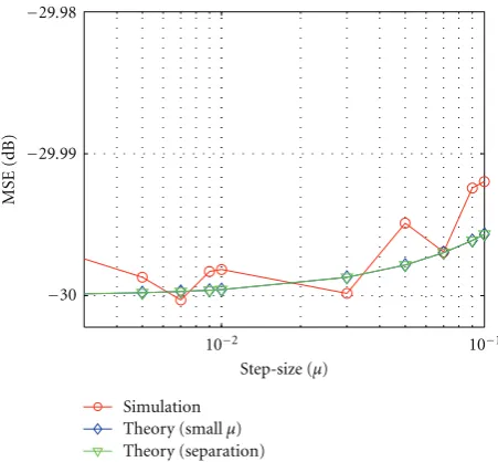
Second, in order to validate the theoretical findings, extensive simulations are carried out for diﬀerent scenarios. While Figures2–4are for the case of the steady-state EMSE of the SRLMF algorithm in a stationary environment,Figure 5

is for the case of the tracking EMSE in a nonstationary

0 2 4 6 8 10 12

×103 −10

−9 −8 −7 −6 −5 −4 −3 −2 −1 0

Iterations

MSE

(dB)

LMF SRLMF

Figure 1: Comparison of the MSE learning curves of LMF and SRLMF algorithms in a uniform noise environment with SNR= 10 dB.

10−2 10−1

−30 −29.99 −29.98

Step-size (µ)

MSE

(dB)

Simulation Theory (small_µ) Theory (separation)

Figure 2: Theoretical and simulated MSE learning curves of the SRLMF algorithm using white Gaussian regressors with shift structure with SNR=30 dB.

environment. In all of these figures the MSE is plotted versus the step-sizeμwith a SNR=30 dB.

In the case ofFigure 2, the regressors, with shift structure, are generated by feeding a unit-variance white process into a tapped delay line. However, inFigure 3, the regressors, with shift structure, are generated by passing correlated data into a tapped delay line. Here, the correlated data are obtained by passing a unit-variance i.i.d. Gaussian data through a first-order autoregressive model with transfer function

√

1−a2_/₍₁₋_az−1_{) and}_a ₌₀_._{8. To further test the validity}

of the results, Gaussian regressors with an eigenvalue spread of five without a shift structure are used, this is depicted in

(10)

10−2 10−1 −30

−29.99 −29.98

Step-size (µ)

MSE

(dB)

Simulation Theory (smallµ) Theory (separation)

Figure3: Theoretical and simulated MSE learning curves of the SRLMF algorithm using correlated Gaussian regressors with shift structure with SNR=30 dB.

10−2 10−1

−30 −29.99 −29.98

Step-size (µ)

MSE

(dB)

Figure4: Theoretical and simulated MSE learning curves of the SRLMF algorithm using Gaussian regressors with an eigenvalue spread=5 without shift structure with SNR=30 dB.

Third, to further validate the theoretical results in a track-ing scenario, the results of Figure 5 depicts this behavior. Here, the random-walk channel behaves according to

wo

i =woi−1+qi, (93)

whereqiis a Gaussian sequence with zero mean and variance σ2

q = 10−9 andwo−1 = wo. As observed fromFigure 5, the

simulation results corroborate closely the theoretical results ((34) and (36)).

Finally, we examine the transient behavior of the SRLMF algorithm for the case of Gaussian data. Let us consider a real-valued regression sequence{ui}with covariance matrix

0 0.01 0.02 0.03 0.04 0.05 0.06 0.07 −35

−30 −25 −20 −15 −10 −5 0

Step-size (µ)

MSE

(dB)

Figure5: Theoretical and simulated MSE learning curves of the SRLMF algorithm for a random-walk channel with SNR=30 dB.

0 2 4 6 8 10

×104 −50

−40 −30 −20 −10 0

Iterations

MSD

(dB)

(a)

0 2 4 6 8 10

×104 −50

−40 −30 −20 −10 0

Iterations

Simulation Theory

MSE

(dB)

(b)

Figure6: Theoretical and simulated MSD (a) and MSE (b) learning curves of the SRLMF algorithm using white Gaussian regressors with SNR=50 dB.

Rwhose eigenvalue spread we set atρ = 5. Let the SNR be 50 dB and the step-size is fixed atμ=0.01.

(11)

0 2 4 6 8 10 ×104 −50

−40 −30 −20 −10 0

Iterations

MSD

(dB)

(a)

0 0

2 4 6 8 10

×104 −50

−40 −30 −20 −10

Iterations

Simulation Theory

MSE

(dB)

(b)

Figure7: Theoretical and simulated MSD (a) and MSE (b) learning curves of the SRLMF algorithm using Gaussian regressors with an eigenvalue spread=5, SNR=50 dB.

9. Conclusions

A new adaptive algorithm, called the SRLMF algorithm, has been presented in this work. Expressions are derived for the steady-state EMSE in a stationary environment. A condition for the mean convergence is also found, and it turns out that the convergence of the SRLMF algorithm strongly depends on the choice of initial conditions. Also, expressions are obtained for the tracking EMSE in a nonstationary environment. An optimum value of the step-size μis also evaluated. Moreover, an extension of the weighted variance relation is provided in order to derive expressions for the mean-square error (MSE) and the mean-square deviation (MSD) of the proposed algorithm during the transient phase. Monte Carlo simulations have shown that there is a good agreement between the theoretical and simulated results. The simulation results indicate that both the SRLMF algorithm and the LMF algorithm converge at the same rate resulting in no performance loss. The analysis developed in this paper is believed to make practical contributions to the design of adaptive filters using the SRLMF algorithm instead of the LMF algorithm in pursuit of the reduction in computational cost and complexity whilst still maintaining good performance.

Acknowledgment

The authors acknowledge the support provided by King Fahd University of Petroleum and Minerals to carry out this work.

References

[1] H. Sari, “Performance evaluation of three adaptive equal-ization algorithms,” inProceedings of the IEEE International Conference on Acoustics, Speech, and Signal Processing (ICASSP ’82), vol. 7, pp. 1385–1389, May 1982.

[2] N. J. Bershad, “On the optimum data nonlinearity in LMS adaptation,”IEEE Transactions on Acoustics, Speech, and Signal Processing, vol. 34, no. 1, pp. 69–76, 1986.

[3] C. P. Kwong, “Dual sign algorithm for adaptive filtering,”IEEE Transactions on Communications, vol. 34, no. 12, pp. 1272– 1275, 1986.

[4] O. Macchi, “Advances in adaptive filtering,” inDigital Com-munications, E. Biglieri and G. Prati, Eds., pp. 41–57, North-Holland, Amsterdam, The Netherlands, 1986.

[5] V. J. Mathews and S. H. Cho, “Improved convergence analysis of stochastic gradient adaptive filters using the sign algorithm,” IEEE Transactions on Acoustics, Speech, and Signal Processing, vol. 35, no. 4, pp. 450–454, 1987.

[6] N. A. M. Verhoeckx and T. A. C. M. Claasen, “Some considera-tions on the design of adaptive digital filters equipped with the sign algorithm,”IEEE Transactions on Communications, vol. 32, no. 3, pp. 258–266, 1984.

[7] E. Eweda, “Almost sure convergence of a decreasing gain sign algorithm for adaptive filtering,” IEEE Transactions on Acoustics, Speech, and Signal Processing, vol. 36, no. 10, pp. 1669–1671, 1988.

[8] E. Eweda, “Tight upper bound of the average absolute error in a constant step-size sign algorithm,”IEEE Transactions on Acoustics, Speech, and Signal Processing, vol. 37, no. 11, pp. 1774–1776, 1989.

[9] T. A. C. M. Claasen and W. F. G. Mecklenbrauker, “Com-parison of the convergence of two algorithms for adaptive FIR digital filters,”IEEE Transactions on Acoustics, Speech and Signal Processing, vol. 29, no. 3, pp. 670–678, 1981.

[10] N. J. Bershad, “Comments on ’comparison of the convergence of two algorithms for adaptive FIR digital filters’,” IEEE Transactions on Acoustics, Speech, and Signal Processing, vol. 33, no. 6, pp. 1604–1606, 1985.

[11] W. A. Sethares, I. M. Y. Mareels, B. D. O. Anderson, C. R. Johnson Jr., and R. R. Bitmead, “Excitation conditions for signed regressor least mean squares adaptation,” IEEE Transactions on Circuits and Systems, vol. 35, no. 6, pp. 613– 624, 1988.

[12] E. Eweda, “Analysis and design of a signed regressor LMS algorithm for stationary and nonstationary adaptive filtering with correlated Gaussian data,”IEEE Transactions on Circuits and Systems, vol. 37, no. 11, pp. 1367–1374, 1990.

[13] S. Dasgupta and C. R. Johnson Jr., “Some comments on the behavior of sign-sign adaptive identifiers,”Systems and Control Letters, vol. 7, no. 2, pp. 75–82, 1986.

[14] S. I. Koike, “Analysis of the sign-sign algorithm based on Gaussian distributed tap weights,” in Proceedings of the IEEE International Conference on Acoustics, Speech and Signal Processing (ICASSP ’98), vol. 3, pp. 1673–1676, May 1998. [15] D. L. Duttweiler, “Adaptive filter performance with

nonlin-earities in the correlation multiplier,” IEEE Transactions on Acoustics, Speech, and Signal Processing, vol. 30, no. 4, pp. 578– 586, 1982.

[16] A. Gersho, “Adaptive filtering with binary reinforcement,” IEEE Transactions on Information Theory, vol. 30, no. 2, pp. 191–199, 1984.

(12)

LMS algorithms,” in Proceedings of the International Sym-posium on Intelligent Signal Processing and Communications (ISPACS ’06), pp. 829–832, December 2006.

[18] A. H. Sayed,Fundamentals of Adaptive Filtering, Wiley Inter-science, New York, NY, USA, 2003.

[19] E. Walach and B. Widrow, “The Least Mean Fourth (LMF) adaptive algorithm and its family,” IEEE Transactions on Information Theory, vol. 30, no. 2, pp. 275–283, 1984. [20] A. Zerguine, C. F. N. Cowan, and M. Bettayeb, “LMS-LMF

adaptive scheme for echo cancellation,”Electronics Letters, vol. 32, no. 19, pp. 1776–1778, 1996.

[21] T. Aboulnasr and A. Zerguine, “Variable weight mixed-norm LMS-LMF adaptive algorithm,” inProceedings of the 33rd Annual Asilomar Conference on Signals, Systems, and Computers, pp. 791–794, Pacific Grove, Calif, USA, October 1999.

[22] M. Moinuddin and A. Zerguine, “Tracking analysis of the NLMS algorithm in the presence of both random and cyclic nonstationarities,”IEEE Signal Processing Letters, vol. 10, no. 9, pp. 256–258, 2003.

[23] A. Zerguine, M. K. Chan, T. Y. Al-Naﬀouri, M. Moinuddin, and C. F. N. Cowan, “Convergence and tracking analysis of a variable normalised LMF (XE-NLMF) algorithm,” Signal Processing, vol. 89, no. 5, pp. 778–790, 2009.

[24] A. Zerguine, M. Moinuddin, and S. A. A. Imam, “A noise constrained least mean fourth (NCLMF) adaptive algorithm,” Signal Processing, vol. 91, no. 1, pp. 136–149, 2011.

[25] R. Price, “A useful theorem for nonlinear devices having Gaussian inputs,”IRE Transactions on Information Theory, vol. 4, no. 2, pp. 69–72, 1958.