Volume 2007, Article ID 95076,11pages doi:10.1155/2007/95076
Research Article
Efficient On-Demand Image Transmission in Visual
Sensor Networks
Kit-Yee Chow, King-Shan Lui, and Edmund Y. Lam
Department of Electrical and Electronic Engineering, The University of Hong Kong, Pokfulam Road, Hong Kong
Received 30 November 2005; Revised 13 September 2006; Accepted 14 September 2006
Recommended by Chun-Shien Lu
In a tracking system, an object of interest is monitored continuously in a sensor network. Information about the object is kept in the sensors and sensors transmit the information upon request. In this paper, we consider the scenario where all sensors around a targeted object capture images of it and these pictures will be sent to a mobile agent upon request. Due to the size and energy limitations in sensors, images kept in sensors are often small and highly compressed. We describe a framework to facilitate a mobile agent in the sensor network to request images of the object of interest. As sensors are limited in energy, it is desirable to reduce the energy used in transmitting the images. We observe that, in a sensor network that is sufficiently dense, images from neighbor cameras would likely overlap, and therefore intermediate sensors can process and combine overlapping portions so as to reduce the energy spent on image transmission. We develop a protocol for involved sensors to determine how to transmit the images they have kept to the mobile agent in an energy efficient manner. Our protocol is truly distributed and does not require any global information. We evaluate our protocol through extensive simulations.
Copyright © 2007 Hindawi Publishing Corporation. All rights reserved.
1. INTRODUCTION
A wireless sensor network consists of thousands of sensors that span a large geographical region. Research and develop-ment in wireless sensor networks are becoming increasingly widespread due to their low cost and low maintenance in de-ployment [1]. These sensors are able to communicate with each other to collaboratively detect objects, collect informa-tion, and transmit messages. Sensor networks have become an important technology especially for environmental moni-toring, target tracking, military applications, disaster man-agement, and so forth [2,3]. A sensor is a very small de-vice and the battery inside is not likely to be rechargeable. This limitation in energy puts extra constraints in the oper-ations of a sensor. In order to prolong its lifetime, a sensor should carefully utilize its energy. Message transmission has been shown to be the major source of energy dissipation. To save energy used in transmission, the size of the messages and the number of messages to be transmitted should be mini-mized. In this paper, we study how images can be processed and transmitted efficiently in terms of energy in a visual sen-sor network.
We consider a tracking system where objects of interest are traced. All sensors are equipped with cameras and they
can take images of a target while it moves inside the sensor network. The images captured are kept in the local memory of the sensors. As sensors are limited in size and therefore have only a small field of view, a camera often can only take a snapshot of a portion of a targeted object. In other words, to get a full view of an object, images captured by several sensors have to be combined before the images can be an-alyzed. In some applications, images of objects in different locations have to be examined at the same time. To reduce the energy consumption in sensors, the analysis will be car-ried out in some powerful nodes instead of in the sensors locally. Traditionally, these powerful nodes are assumed to be fixed servers wired with power cable sitting at the rim of the sensor network. An image is sent to these fixed servers in a hop-by-hop manner. As a server is at a peripheral position, the paths from the sensors in the central area of a network can be very long, especially when the sensors span a large ge-ographical area. This is not energy efficient since images are large in size and several images are needed for a single ob-ject.
sending images to a fixed server, sensors relay their pictures to this mobile sink. There are several issues that have to be addressed when data are sent to a mobile node instead of a fixed one. First, since the sink is now mobile, it also has en-ergy concern. That is, if we keep on sending pictures to the sink, the sink may get overwhelmed and some pictures will be lost due to insufficient energy or memory. Second, when the sink is fixed, sensors can be preconfigured with its location and every sensor will know where to send its images. This does not apply when the sink becomes mobile. A mechanism that allows a sensor to locate the sink is needed.
To solve the two problems, we take an on-demand re-quest approach. The mobile sink sends out rere-quests to sen-sors when it wants to collect the images. In this way, the mobile sink can estimate how much information it can han-dle and makes requests accordingly. The possibility of over-whelming is highly reduced. On the other hand, the mo-bile sink should also put its location in the request messages. Sensors can then know where to send their pictures without much extra overhead.
After receiving a request, sensors that have images of the same target will send their images to the mobile sink. Since they may overlap with each other, intermediate sensors on the path from the cameras to the mobile sink can combine images of overlapping regions so as to reduce the size of the images. Different paths may have different hop counts and images can be combined in different ways. In this paper, we investigate how to optimize the energy resources in transmit-ting images on demand to a mobile node through selectransmit-ting appropriate paths. We develop a distributed protocol that helps to reduce the total transmission energy. We evaluate our protocol through extensive simulations and the simula-tion results show that our protocol, when compared to send-ing images individually, can achieve a significant reduction in energy usage without any additional computational cost.
The rest of the paper is organized as follows.Section 2 presents the related work.Section 3 describes the network model.Section 4describes the protocol, and the simulation results are shown inSection 5. We finally conclude our paper inSection 6.
2. RELATED WORK
A sensor node can reduce the energy spent in transmission by combining the data it receives from neighbors together before transmitting it out. For example, if the sensors are transmitting the average temperature of the area they reside in, when a sensor receives two averagesA1 andA2 from two neighbors, it can calculate (A1 +A2)/2 and send it out. Two or more messages can be “combined” into one message and transmission energy is saved. The process of combining sev-eral messages into one is calleddata aggregation. The prob-lem of finding optimal data aggregation has been proved to be NP-hard [5,6]. Some mechanisms have been developed to aggregate simple scalars [7–10], but only a few of them study the employment of aggregation of more complex data types. Data aggregation can also be applied to visual sensor net-works, but the multimedia nature of the data presents extra
challenges in designing a proper mechanism for aggregation. Several recent studies tackle various aspects of this problem. Reference [11] shows that applying maximum compression before transmission does not necessarily minimize the to-tal energy used. The authors then develop a heuristic for selecting a good compression level based on global infor-mation. Yu et al. [12] develop a mechanism for transmit-ting JPEG2000 images in one hop. Given an expected im-age quality, the algorithm’s objective is to minimize the en-ergy spent in processing and transmission. Reference [13] studies distributed image compression, where the compu-tation in wavelet transform and quantization of subbands in JPEG2000 are shared among different groups of sensor nodes. This approach does not aim at decreasing the total energy needed, but because each sensor only accounts for a part of the computation, the maximum energy needed in a sensor is reduced. Reference [14] also studies distributed image compression, but from a different perspective. In this setting, each sensor captures a low-resolution image of the object, and assuming that overlapping areas across images from different sensors can be identified, super-resolution of these low-resolution images is performed at the receiver. The approach in [15] uses geometrical information to estimate the correlation of visual images of the same object and to determine how to compress the images. Reference [16] de-scribes a camera network where sensors are organized hier-archically into several tiers. Lower power cameras are at the bottom and they are capable of taking low-resolution im-ages. When an object of interest is identified, these sensors can trigger cameras in a higher tier on demand to get better images.
None of the work mentioned above considers the effect of using different paths in transmitting the images. SPIN-IT [17] is a routing protocol for retrieving an image based on metadata of images. It focuses on how a node iden-tifies the sources of an image requested but not the im-age transmission issues. In our earlier work [18, 19], we demonstrate that when there is overlap in the scene cap-tured by the cameras, and intermediate processing is pos-sible to combine the images, the image transmission strat-egy is nontrivial. Under different ratios of transmission and compression energy, we develop guidelines that stipulate dif-ferent routes for transmitting images in order to minimize the overall energy used in the system. We assume that the server is fixed and only a few sensors can aggregate images in [18]. In this paper, we consider a more general problem that images are sent to a mobile sink and all sensors are equal in that they all can capture, aggregate, and transmit images.
3. NETWORK MODEL
S
+
Figure1: A simple network.
neighbors. All sensors are identical in terms of their capabil-ities in handling the images.
3.1. Tracking and image capture
In our system, the main task of the sensors is to take images of a certain targeted object and transmit them to a mobile sink upon request. The object of interest moves around in the sensor network. When a sensor detects that the object is nearby, it determines whether to take a picture of it or not. Since a sensor network is dense, many sensors can sense the same object simultaneously. We let these sensors coordi-nate with each other to take pictures at about the same time. Time synchronization can be done through GPS or a clock synchronization algorithm [21]. On the other hand, as these sensors are collaborating to track the object, a sensor should also realize whether its image overlaps with its neighbor’s im-age and to what extent. It is possible that imim-ages captured do not overlap. It is also possible that some images contain over-laps but some do not. Whether the sensors want to capture overlapping images depends on the application requirement. Our protocol works for situations that may contain overlap-ping and nonoverlapoverlap-ping images.
Referring to the network inFigure 1where the object of interest is represented as “+,” the white nodes are the sen-sors that will capture images of the object. In a typical track-ing system, the sensors should also record the time that the pictures are taken and the object involved. The images cap-tured are kept in the local memory of sensors. Upon request, the images are then sent to the mobile sink. As the mobile sink may not request images frequently, a sensor may have taken pictures of several different targets before the mobile sink makes a request. To reduce the size of the images, images are compressed and saved in the local memory of a sensor. In our system, we use JPEG compression, but we also note that JPEG2000 and other proprietary schemes may also be used in similar settings.
3.2. Mobile sink
A mobile sink is a mobile node in the network that collects images on demand. It can appear in different locations to col-lect information. When it decides to colcol-lect images, it sends out a request that specifies what images it wants. For exam-ple, in a wild life surveillance application, the request can be
“Please give me the pictures of a tiger captured at 1:00 AM today.” This request also contains the information about the mobile node and a hop count (hc) field to keep track of how far this request has traveled.hc is initialized to 1. Since the mobile sink does not know which sensors have the informa-tion it wants, this request is flooded to all the nodes in the network. To simplify our discussion, we assume that the mo-bile sink will remain static until the requested images are ceived or the mobile sink foresees that there will be no re-ply. Since the mobile sink should not be a fast moving node, if it moves after sending out the request, the nodes near its original location can collect the images and send them to the new location of the mobile sink, which should not be very far away.
3.3. Request handling
A request is flooded to all the nodes in the network. There-fore, every sensor would receive the request at least once. Nodes that possess the required images should therefore send their stored images to the mobile sink. The image transmis-sion will be described inSection 4in detail. In this section, we focus on discussing how nodes handle the request messages for developing forwarding paths towards the mobile sink.
When a noden receives a request for the first time, it should record how far away it is from the mobile sink in terms of hop count.hccarried in the request specifies how many hopsnis from the mobile sink.nalso keeps track that the hop count from the mobile sink to the neighbor ishc.n then incrementshcby one and sends the request to its neigh-bor. It is possible thatnreceives the same request more than once since more than one of its neighbors send out the re-quest. Ifnreceives another copy of the request from neigh-borb and the hop count in the request ishc(b), it records this information in the database. It does not resend the re-quest again. After all the copies are handled,nshould know
(i) the location of the mobile sink,
(ii) its distance, in terms of hop count, to the mobile sink, (iii) for each neighborb, the distance between the mobile
sink andb.
As the mobile sink does not station in a location forever, the record about a request should be cleared after some time.
4. PROTOCOL
Apart from updating the hop count and neighbor informa-tion, a node should also note whether it possesses the image requested. In this section, we will describe how sensors trans-mit the requested images to the sink. We first go over some notations.
4.1. Notations
To facilitate our discussion, we adopt the following notations andFigure 2illustrates some of them.
Ii JPEG compressed image kept at camerai.
Ii
i j The portion ofIithat overlaps withIj.
Ii Ii ji The portion ofwithI Iithat does not overlap j.
IiIj
Resultant image after stitchingIiandIj if they overlap.
I Size of imageI.
Et Energy needed in transmitting unit byteto a neighbor.
Ec Energy needed in compressing/decompressingunit byte.
Ea Energy needed in performing image alignmentper byte.
hc(n) Hop count of noden.
NB(n) Neighbor set of noden.
4.2. Determination of overlapping portions
By making use of an image-based localization algorithm such as in [22,23], the physical locations and orientations of cam-era nodes can be known. We take the viewpoint of these pa-pers that the overlapping portions among images can be de-duced geometrically [24], and the energy involved in identi-fying the overlapping regions is small compared to the other processes in the sensor network. If the two images differ in scale, angle, or other parameters, we would need further im-age alignment on these visual data [25], that is, establishing the mathematical relationships that map pixel coordinates from one image to another, before performing data aggre-gation.
In sensor networks, the camera nodes are reasonably close to each other. We may assume that the magnifications and points of view among neighbor images are similar. The number of parameters involved in image alignment is thus small, and the energy consumption needed in performing image alignment would be manageable for a sensor node [26]. In truly random distribution of sensor nodes in 3D, the image alignment would be much more complicated. To facil-itate our discussion, we consider the simpler scenario.
4.3. Transmission of two neighboring images
Consider that camerasiandj are neighbors and they both want to send their images,IiandIj, to the mobile sink,S. If
Iiis transmitted individually toSin a hop-by-hop manner, the transmission load needed ishc(i)Ii. If bothIiandIj are sent independently, the total transmission load (number of bytes to be transmitted)Tdumrequired is
Tdum=hc(i)Ii+hc(j)Ij. (1)
In a dense network, it may happen thatIioverlaps with several other images captured in other cameras. Since the cameras take images in a collaborative manner, we can as-sume that each portion ofIioverlaps with at most one more neighbor image. That is, each portion can aggregate with at most one other image. In other words, we can partition Ii into several regions where some regions can be aggregated with exactly one neighbor image while some regions do not overlap with any image. For example, in Figure 2, Ii ji is the portion ofIithat overlaps withIj and (Ii Ii ji ) is the
Ii Ij
Ii
Ii Ii ji Ii ji
Figure2: Illustration ofIi ji andIi Ii ji .
nonoverlapping region ofIi. These regions will be sent inde-pendently.
Suppose thatIiandIjoverlap with each other, soIi ji =
andI j
i j =. After receiving the images, it could be ad-vantageous for S to decompress the overlapping region in both images, average them, and recompress the region, in or-der to save on the amount of image data needed for further transmission. The averaging is performed to reduce the re-sulting amount of noise; if the captured images already pos-sess good signal-to-noise ratios (SNR), we may not need the averaging but only choose to send one of the two copies of the same scene. We denote the raw image of an JPEG image
I to beR(I). LetCbe the decompression/compression load and let Abe the image alignment load of performing data aggregation. We have
C=RIi
i j+RIiJj+R
Iij,
A=RIi
i j,
(2)
whereIi jis the overlapping region after averaging. Note that
R(I i
i j)=R(I j
i j)=R(Ii j).
Since all sensors are able to perform image processing functions, transmission energy can in fact be reduced by al-lowing intermediate sensors on the path to combine the over-lapping region. For example, ifiandjboth send their images to neighbor node ktowards Sas shown inFigure 3,kcan also decompressIi ji andIi jj to formIi j. The energy spent is exactly the same as the operation done inS. Nevertheless, we save transmission energy. Suppose thathc(i)= hc(j) =
hc(k) + 1, the total transmission loadTnow is
T=Ii+Ij+hc(k)IiIj. (3)
We can see that
Tdum=hc(k)Ii+Ii+hc(k)Ij+Ij
> hc(k)IiIj+Ii+Ij=T.
(4)
In other words, energy is saved as we apply image aggre-gation in intermediate sensor nodes when images overlap.
s
Ii Ij
k
Ii Ij
i j
Figure3: Aggregating images at a common neighbor.
(1)hc(i)=hc(j)
i recordshc(i) when it receives a request sending from its neighborkwherehc(k)=hc(i) 1.kis also a neighbor lying on the shortest path towardsS. There are two subcases.
(a) There exists a nodekwhich is the common neighbor of iand j; in other words, k NB(i)NB(j) and
hc(k)=hc(i) 1.
(b) There does not exist a nodeksuch thatk NB(i)
NB(j) andhc(k)=hc(i) 1. In this case, the next hop neighbors lying on the shortest paths toSforiandj are different. We label themkiandkj.
(2)hc(i)=hc(j)
In this case,hc(i) andhc(j) can differ by at most 1 sinceiand
j are neighbors. Without loss of generality, we assume that
hc(j)=hc(i) 1. Note that jcan be a next hop neighbor of
ileading toS.
We now describe the most energy efficient way to ag-gregate images that take into account the 3 scenarios. An important feature of our mechanism is that it does not re-quire global information and bothiandjcan make decisions based on its own information in a distributed manner.
Case 1. This is the situation depicted in Figure 3.i and j should send their images to a common neighbor k and k stitches them to form IiIj. To identifyk,i should check for eachb NB(i) wherehc(b) = hc(i) 1, whether bis inNB(j) as well. Sinceiknows its neighbors and their hop counts fromS,ican find out b b NB(i) andhc(b) =
hc(i) 1easily. To determine whetherb NB(j),i com-putes the physical distance betweenbandjusing their loca-tions. If the distance is smaller than the range of transmis-sion,bis also a neighbor ofj. It is possible that there are sev-eral neighbors satisfying the conditions butiandjshould se-lect the same one to send their images. A simple tie breaking mechanism is to use energy level. The neighbors with highest energy level are selected ask. Nodekis then responsible for performing image alignment and data aggregation.
S
ki kj
i j
Ii Ii ji Ii ji Ij
IiI i i j
Ii i j
Ii
i j Ij
Figure4: Aggregating images at nodej.
MAIN
1: if (hc(i)=hc(j))
2: {ifkNB(i)NB(j) ANDhc(k)=hc(i) 1
3: {
4: Iikfromi;
5: Ijkfromj;
6: IiIjSfromk;
7: }
8: else{
9: SEND2(i,j);
10: }
11: endif;
12: }
13: else
14: {if (hc(i)> hc(j))
15: {
16: SEND2(i,j);
17: }
18: else SEND2(j,i);
19: }
20: endif;
Algorithm1
Case 2. iandjknow whether they have any common neigh-borkwherehc(k)=hc(i) 1 by using the same mechanism as described inCase 1. Sincekdoes not exist, ifiand j sim-ply send their images to a next hop neighbor leading toS, it is not guaranteed thatIiandIjcan be aggregated. Therefore, our protocol requires eitherior jto send its overlapping re-gion to the other node. That is, ifiis of lower energy level,
isendsIi ji to j and sendsIi Ii ji to ki. This is shown in Figure 4. Node jis responsible for performing image align-ment and data aggregation.
Case 3. Without loss of generality, we lethc(j)=hc(i) 1.i should sendIi ji tojand sendIi Ii ji to another neighborki ifhc(ki)=hc(j). In fact, the energy spent here is the same as sending the wholeIito j. We breakIiinto two portions and use different paths because we can reduce the transmission energy used in j. This is also depicted inFigure 4.
SEND2(i,j)
1:Ii ji jfromi;
2:Ii Ii jI Sfromi;
3:Ii j+ (Ij Ii jj )Sfromj;
Algorithm2
4.4. Transmission energy and computational energy
The transmission loadT, compression/decompression load
C, and image alignment loadAof different cases are the fol-lowing.
Case 1
T=Ii+Ij+IiIjhc(k),
C=3R
Ii j,
A=RIi j.
(5)
Cases2and3
T=Ii
i j+Ii Ii ji hc(i) +I i
i jIjhc(j),
C=3R
Ii j,
A=RIi j.
(6)
4.5. Example
Suppose the area covered by the network is divided into
mmgrids and the location of each grid is represented as (row, col). The camera nodes are distributed randomly in the network and each grid contains at most one node. For ex-ample, inFigure 5, the “+” represents the object of interest and the numbers indicate the hop count of each node. Only those inside the dashed rectangle will capture the images of the object. In this scenario, the object of interest is located at (11, 13) and there are 13 nodes that are responsible for cap-turing images. They are divided into 8 groups as circled in Figure 5. For the group of nodes at (11, 11) and (10, 11), the hop counts of both nodes are 4. We want to find a nodek such thatk NB(i)NB(j) andhc(k) = hc(i) 1. By searching in the network, we can identify several neighbors that satisfy this condition and the neighbor with the highest energy level is selected ask. In this case,kis located at (9, 10) withhc(k) = 3. Let the nodes at (11, 11) and (10, 11) bei and j, respectively, and the corresponding images beIiand
Ij,iandjwill send their images tokand thenkwill perform image alignment and stitch them to formIiIj. The total energy consumptionETotal
pro for this group will be
T=Ii+Ij+ 3IiIj,
C=3R
Ii j,
A=RIi j,
ETotal
pro =TEt+CEc+AEa.
(7)
Col
10 11 12 13 14 15 16 Row
8 9 10 11 12 13 14
3 5
4 4 4 5 6
4 + 6 6
5 5 5 6
5 5 6 6 6
6 6
6
5 5
4 4 3
Figure5: Object of interest.
1 1
1 1 1 S 1
1 1
2 2 2
2
Figure6: Neighbor nodes ofS.
5. SIMULATION
In this section, we present our simulation results that show that the protocol is beneficial in reducing the total transmis-sion energy. The simulation results are generated using MAT-LAB. Network topologies are generated randomly. The whole area is divided intoNNgrids. There is at most one sensor in each grid and the probability that a grid has a sensor de-pends on the density and is generated randomly. The mobile sinkScan appear anywhere in the network. The transmis-sion range is 3.535, which covers the neighboring 55 grids. For example, any nodes inside the window withSas center are the neighbors ofS, and the hop count of those neighbor nodes are one,hc(n)= 1. Similarly, the neighbor nodes of nodenwithhc(n) = 1 will have hop counts equal to two. The hop counts of all the nodes in the network are assigned in this manner. In the example shown inFigure 6,Sindicates the mobile sink and the numbers indicate the hop count of each node.
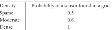
Table1
Density Probability of a sensor found in a grid
Sparse 0.3
Moderate 0.6
Dense 1
It is also possible that the image does not overlap with any other image. In this case, the sensor will send its image di-rectly back to the mobile sink along the shortest path. For the grouped nodes, they will send their images according to the protocol proposed in the previous section.
In our simulation, the network size is set to be a 5050 grid, the mobile sink and the object of interest can be at any grid. LetDbe the distance between the object of interest and the mobile sink. We consider five different cases:
(1) 0D <5, (2) 5D <10, (3) 10D <15, (4) 15D <20, (5) 20D <25.
Each case is simulated with three different densities of nodes: dense, moderate, and sparse. The relationship be-tween density and probability that a grid has sensor is as shown inTable 1. There are 3 different densities and 5 dif-ferent ranges of distance, so 15 combinations can be formed. Each combination is simulated 20 times to calculate the av-erage reduction in transmission energy.
The total energy consumed in each case is compared with the dummy case, that is, each node sends the image indepen-dently along its shortest path. LetETotal
pro be the total energy consumed in tested case, letETotal
dum be the total energy con-sumed in the dummy case, and letEdiff be the energy diff er-ence.
If we assume the mobile sink will perform data aggrega-tion on the received images, the energy equaaggrega-tions will be
ETotal pro =
TEt+
CEc+
AEa, (8)
ETotal dum =
TdumEt+
CEc+
AEa,
Ediff = T
dum
TEt.
(9)
Since the computational load of both cases is the same, the total energy consumption difference is equal to the transmis-sion load difference.Figure 7shows the percentage change of transmission load which is calculated by
change (%)=
Tdum
T
Tdum
100%. (10)
In our simulation, the percentage change is always pos-itive which shows that the total transmission energy
con-0 5 10 15 20 25
R
eduction
in
tr
ansmission
energ
y
(%)
Sparse Moderate density
Dense
0 D <5 5 D <10 10 D <15
15 D <20 20 D <25
Figure7: Reduction in transmission energy.
sumed by using the protocol is always less than that con-sumed in the dummy case. The results with different com-bination of object distance and sensor density are shown in Figure 7. From the result, we can observe that the reduction in transmission energy is greater when the object is farther away fromS. Additionally, the reduction will be more signif-icant as the density increases. When the network is denser, the camera nodes are closer to each other and thus the im-age overlaps with its neighbor’s imim-age to a greater extent. The greater the overlapping portion is, the more the energy is saved. The energy saved by applyingCase 1or isCase 2of the protocol isI
i
i jhc(k)Etand the energy saved inCase 3is
I j
i jhc(j)Et. WhenI i
i jandI j
i jincrease, the energy saved will also increase.
If we assume the mobile sink will not perform data ag-gregation on the received images,ETotal
pro will be the same as (8) butETotaldumwill be different. The energy equations will be
ETotal dum =
TdumEt,
Ediff= T
dum
TEt
CEc
AEa.
(11)
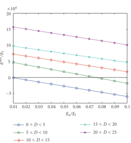
In Figures8–10, thex-axis represents Ea/Et and the y -axis represents the normalized energy difference between our protocol and the dummy case, that is,Ediff/Et. For the nor-malized energy difference,
Ediff
Et = Tdum
T C
Ec
Et
A
Ea
4 2 0 2 4 6 8 10 12 14
0.01 0.02 0.03 0.04 0.05 0.06 0.07 0.08 0.09 0.1 104
Ea/Et
E
di
ff/E
t
0D <5 5D <10 10D <15
15D <20 20D <25
Figure8: Sparsely populated network.
5 0 5 10 15 20
0.01 0.02 0.03 0.04 0.05 0.06 0.07 0.08 0.09 0.1 104
Ea/Et
E
di
ff/E
t
0D <5 5D <10 10D <15
15D <20 20D <25
Figure9: Moderately populated network.
In addition toEa/Et,Ec/Et is also a factor in the above equation. Reference [27] claims that communication/com-putation power usage ratio can be higher than 1000, and thus
Ec/Etcan be as small as 0.001. To allow for different applica-tions where this number can vary, we take a more conserva-tive estimate and setEc/Etequal to 0.005. With this assump-tion, we can estimate the relationship between normalized total energy difference and normalized energy needed in per-forming image alignment.
1.5 1 0.5 0 0.5 1 1.5 2 2.5 3 3.5
0.01 0.02 0.03 0.04 0.05 0.06 0.07 0.08 0.09 0.1 105
Ea/Et
E
di
ff/E
t
0D <5 5D <10 10D <15
15D <20 20D <25
Figure10: Densely populated network.
When the normalized energy difference is positive that means the total energy consumption in dummy case is greater than that in our protocol, and vice versa. The crossing points on the zero-axis are the critical values ofEa/Et. If the ratio is smaller than the critical value, our protocol will be more energy efficient than sending the images independently along their shortest paths.
When the density increases, the critical value increases. A higher critical value means the protocol can tolerate a larger computational energy for image alignment. As the density increases, the amount of overlapping portions also increases. Since transmission energy is far greater than computational energy, the reduction in total transmission energy consump-tion is much more significant than the increase of total com-putational energy dissipation.
On the other hand, the critical value increases as the ob-ject of interest moves away from the sink under the same density. This indicates that the protocol can tolerate a higher processing cost for image alignment. This is reasonable be-cause more transmission energy is saved as the object is far-ther away, and far-therefore the protocol can bear a larger com-putational cost.
Figure 11shows the result of sparsely populated density network with size of 2020 grids. By comparingFigure 11 withFigure 8, it can be observed that the two plots are very similar. The only difference is for the curve 20 D < 25, because for a 2020 grid, the object of interest would be lo-cated at the margin of the network. Thus, we can see that the advantage of our protocol holds for different network sizes.
It is easy to verify that the transmission energy saved by applyingCase 1orCase 2of the protocol isI
i
i jhc(k)Et and the energy saved inCase 3isI
j
4 2 0 2 4 6 8 10 12
0.01 0.02 0.03 0.04 0.05 0.06 0.07 0.08 0.09 0.1 104
Ea/Et
E
di
ff/E
t
0D <5 5D <10 10D <15
15D <20 20D <25
Figure11: Sparsely populated network, network size=2020.
we can approximate the ratio between the size of raw image data and the size of compressed image. LetM be the ratio betweenR(I
i
i j)andI i
i j. The computation load for each case of the protocol becomes
C=3MI
i i j,
A=MI
i i j.
(13)
The normalized energy difference forCase 1orCase 2will be
Ediff
Et =
Ii
i jhc(k) 3MI i i j
Ec
Et
MI
i i j
Ea
Et.
(14)
The normalized energy difference forCase 3will be
Ediff
Et =
Ii
i jhc(j) 3MI i i j
Ec
Et
MI
i i j
Ea
Et.
(15)
SinceEt,Ec,Ea, and hop count can also be known, each pair of nodes can determine whether to send their images ac-cording to the protocol or not by calculating the approximate value of energy difference. IfEdiff >0, the images should be sent according to the protocol or else the images should be
sent independently along their shortest paths:
0< E diff
Et
=Ii
i j
hc(κ) 3M
Ec
Et M
Ea
Et
=hc(κ) 3M
Ec
Et M
Ea
Et,
(16)
where
κ=
⎧ ⎨ ⎩k
Case1or2,
j Case 3. (17)
Reference [28] claims that the image quality of a compressed image with compression ratio of 32-to-1 is considered to be good. In our simulation, the ratio between the size of raw image data and the size of compressed image,M, is about 35. The hop count of a node which captured the image of the object of interest in the range 0–5 unit away from the sink in a sparsely populated network is in the range of 1–3, and we assumeEc/Et to be 0.005. By plugging the parameters into (16), we can find that the estimated critical value ofEa/Et is around 0.0405. This value is different from the crossing point onFigure 8, since that is the overall energy difference plot which contains several pairs of nodes and the value ofM is image dependent. Although we cannot predict the energy difference precisely, the approximation gives a good indica-tion for the node to determine the path to send the image.
6. CONCLUSION
In this paper, we investigate how to optimize the energy re-sources in transmitting images on demand to a mobile node through selecting appropriate paths. A distributed protocol was proposed and evaluated through extensive simulations. Depending on the ratios of transmission and computational energy, network density, compression level, and object dis-tance, the sensors should choose to send the images accord-ing to the protocol or not.
It should be noted that the assumptions used in this work have room for refinement, especially when the methodology is applied to applications where the overlapping among im-ages may not be easily determined. Examples include track-ing objects without strongly identifiable features while re-quiring strictly image-based localization. Similar to most of the related works, in this paper we assume that the overlap-ping regions among images can be deduced by the geometric positions of the sensors. One direction for our future work is to develop an explicit solution in identifying the overlapping among images using advanced vision-based approaches.
ACKNOWLEDGMENTS
University Grants Committee, Hong Kong Special Admin-istrative Region, China, Project no. HKU 7147/04E and the Small Project Funding, established by the University of Hong Kong, Project no. 200507176083.
REFERENCES
[1] F. Zhao and L. Guibas,Wireless Sensor Networks: An Informa-tion Processing Approach, Morgan Kaufmann, San Francisco, Calif, USA, 2004.
[2] D. Estrin, D. Culler, K. Pister, and G. Sukhatme, “Connecting the physical world with pervasive networks,”IEEE Pervasive Computing, vol. 1, no. 1, pp. 59–69, 2002.
[3] G. J. Pottie and W. J. Kaiser, “Wireless integrated network sen-sors,”Communications of the ACM, vol. 43, no. 5, pp. 51–58, 2000.
[4] W. Wang, V. Srinivasan, and K.-C. Chua, “Using mobile relays to prolong the lifetime of wireless sensor networks,” in Pro-ceedings of the 11th Annual International Conference on Mo-bile Computing and Networking (MobiCom ’05), pp. 270–283, Cologne, Germany, August-September 2005.
[5] B. Krishnamachari, D. Estrin, and S. Wicker, “The impact of data aggregation in wireless sensor networks,” inProceedings of the IEEE International Workshop on Distributed Event-Based Systems (DEBS ’02), pp. 575–578, Vienna, Austria, July 2002. [6] C. Buragohain, D. Agrawal, and S. Suri, “Power aware routing
for sensor databases,” inProceedings of the IEEE 24th Annual Joint Conference of the IEEE Computer and Communications Societies (INFOCOM ’05), vol. 3, pp. 1747–1757, Miami, Fla, USA, March 2005.
[7] M. Ding, X. Cheng, and G. Xue, “Aggregation tree construc-tion in sensor networks,” inProceedings of the IEEE 58th Vehic-ular Technology Conference (VTC ’03), vol. 4, pp. 2168–2172, Orlando, Fla, USA, October 2003.
[8] N. Shrivastava, C. Buragohain, D. Agrawal, and S. Suri, “Me-dians and beyond: new aggregation techniques for sensor net-works,” inProceedings of the 2nd International Conference on Embedded Networked Sensor Systems (SenSys ’04), pp. 239– 249, Baltimore, Md, USA, November 2004.
[9] S. Nath, P. B. Gibbons, S. Seshan, and Z. R. Anderson, “Syn-opsis diffusion for robust aggregation in sensor networks,” inProceedings of the 2nd International Conference on Embed-ded Networked Sensor Systems (SenSys ’04), pp. 250–262, Bal-timore, Md, USA, November 2004.
[10] J.-Y. Chen, G. Pandurangan, and D. Xu, “Robust computation of aggregates in wireless sensor networks: distributed random-ized algorithms and analysis,” inProceedings of the 4th Interna-tional Symposium on Information Processing in Sensor Networks (IPSN ’05), pp. 348–355, Los Angeles, Calif, USA, April 2005. [11] H. Wu and A. A. Abouzeid, “Power aware image transmission
in energy constrained wireless networks,” inProceedings of the International Symposium on Computers and Communications (ISCC ’04), vol. 1, pp. 202–207, Alexandria, Egypt, June-July 2004.
[12] W. Yu, Z. Sahinoglu, and A. Vetro, “Energy efficient JPEG 2000 image transmission over wireless sensor networks,” in
Proceedings of the IEEE Global Telecommunications Conference (GLOBECOM ’04), vol. 5, pp. 2738–2743, Dallas, Tex, USA, November-December 2004.
[13] H. Wu and A. A. Abouzeid, “Energy efficient distributed JPEG2000 image compression in multihop wireless networks,”
inProceedings of the 4th Workshop on Applications and Services in Wireless Networks (ASWN ’04), pp. 152–160, Boston, Mass, USA, August 2004.
[14] R. Wagner, R. Nowak, and R. Baraniuk, “Distributed image compression for sensor networks using correspondence anal-ysis and super-resolution,” inProceedings of the IEEE Interna-tional Conference on Image Processing (ICIP ’03), vol. 1, pp. 597–600, Barcelona, Spain, September 2003.
[15] N. Gehrig and P. L. Dragotti, “Distributed compression in camera sensor networks,” inProceedings of the IEEE 6th Work-shop on Multimedia Signal Processing, pp. 311–314, Siena, Italy, September-October 2004.
[16] P. Kulkarni, D. Ganesan, P. Shenoy, and Q. Lu, “SensEye: a multi-tier camera sensor network,” inProceedings of the 13th ACM International Conference on Multimedia (ACM Multime-dia ’05), pp. 229–238, Singapore, November 2005.
[17] E. Woodrow and W. Heinzelman, “SPIN-IT: a data centric routing protocol for image retrieval in wireless networks,” in
Proceedings of the IEEE International Conference on Image Pro-cessing (ICIP ’02), vol. 3, pp. 913–916, Rochester, NY, USA, September 2002.
[18] K.-S. Lui and E. Y. Lam, “Image transmission in sensor net-works,” inProceedings of the IEEE Workshop on Signal Process-ing Systems (SiPS ’05), pp. 726–730, Athens, Greece, November 2005.
[19] K.-Y. Chow, K.-S. Lui, and E. Y. Lam, “Balancing image quality and energy consumption in visual sensor networks,” in Pro-ceedings of the 1st International Symposium on Wireless Perva-sive Computing (ISWPC ’06), pp. 1–5, Phuket, Thailand, Jan-uary 2006.
[20] X. Ji and H. Zha, “Sensor positioning in wireless ad-hoc sen-sor networks using multidimensional scaling,” inProceedings of the 23rd IEEE Annual Joint Conference of the IEEE Com-puter and Communications Societies (INFOCOM ’04), vol. 4, pp. 2652–2661, Hong Kong, March 2004.
[21] Q. Li and D. Rus, “Global clock synchronization in sensor net-works,” inProceedings of the 23rd Conference of the IEEE Com-puter and Communications Societies (INFOCOM ’04), vol. 1, pp. 564–574, Hong Kong, March 2004.
[22] H. Lee and H. Aghajan, “Vision-enabled node localization in wireless sensor networks,” inCOGnitive Systems with Interac-tive Sensors (COGIS ’06), Paris, France, March 2006.
[23] C. McCormick, P.-Y. Laligand, H. Lee, and H. Aghajan, “Dis-tributed agent control with self-localizing wireless image sen-sor networks,” inProceedings of the Conference on COGnitive Systems with Interactive Sensors (COGIS ’06), Paris, France, March 2006.
[24] H. Ma and Y. Liu, “Correlation based video processing in video sensor networks,” inProceedings of the International Confer-ence on Wireless Networks, Communications and Mobile Com-puting (ICWN ’05), vol. 2, pp. 987–992, Las Vegas, Nev, USA, June 2005.
[25] H. S. Sawhney and R. Kumar, “True multi-image alignment and its application to mosaicing and lens distortion correc-tion,”IEEE Transactions on Pattern Analysis and Machine In-telligence, vol. 21, no. 3, pp. 235–243, 1999.
[27] V. Raghunathan, C. Schurgers, S. Park, and M. B. Srivastava, “Energy-aware wireless microsensor networks,” IEEE Signal Processing Magazine, vol. 19, no. 2, pp. 40–50, 2002.
[28] B. G. Haskell, P. G. Howard, Y. A. LeCun, et al., “Image and video coding-emerging standards and beyond,”IEEE Transac-tions on Circuits and Systems for Video Technology, vol. 8, no. 7, pp. 814–837, 1998.
Kit-Yee Chow received her B.Eng. (first class honors) degree from the University of Hong Kong in 2005. She is currently pursu-ing the M.Phil. degree at the Department of Electrical and Electronic Engineering, The University of Hong Kong. Her research in-terests are in the areas of sensor networks and image processing.
King-Shan Lui obtained her B.Eng. (first class honors) and M.Phil. degrees in com-puter science from The Hong Kong Uni-versity of Science and Technology. She then received her Ph.D. degree, also in com-puter science, from the University of Illi-nois at Urbana-Champaign, USA, in 2002. She joined the Department of Electrical and Electronic Engineering, The University of Hong Kong, as an Assistant Professor in
Au-gust 2002. Her research interests include computer network quality of service issues, protocol and algorithm design in the Internet, ad hoc networks, and sensor networks.
Edmund Y. Lamreceived the B.S. degree (with distinction) in 1995, the M.S. de-gree in 1996, and the Ph.D. dede-gree in 2000, all in electrical engineering from Stanford University, Stanford, Calif. At Stanford, he developed image processing algorithms for the Programmable Digital Camera project. He also consulted for industry in the ar-eas of digital camera systems design and al-gorithms development. Before returning to