Time–frequency based feature selection for discrimination of non-stationary biosignals

R E S E A R C H

Open Access

Time–frequency based feature selection for

discrimination of non-stationary biosignals

Juan D Mart´ınez-Vargas

, Juan I Godino-Llorente

and Germ´an Castellanos-Dominguez

Abstract

This research proposes a generic methodology for dimensionality reduction upon time–frequency representations applied to the classification of different types of biosignals. The methodology directly deals with the highly redundant and irrelevant data contained in these representations, combining a first stage of irrelevant data removal by variable selection, with a second stage of redundancy reduction using methods based on linear transformations. The study addresses two techniques that provided a similar performance: the first one is based on the selection of a set of the most relevant time–frequency points, whereas the second one selects the most relevant frequency bands. The first methodology needs a lower quantity of components, leading to a lower feature space; but the second improves the capture of the time-varying dynamics of the signal, and therefore provides a more stable performance. In order to evaluate the generalization capabilities of the methodology proposed it has been applied to two types of biosignals with different kinds of non-stationary behaviors: electroencephalographic and phonocardiographic biosignals. Even when these two databases contain samples with different degrees of complexity and a wide variety of characterizing patterns, the results demonstrate a good accuracy for the detection of pathologies, over 98%. The results open the possibility to extrapolate the methodology to the study of other biosignals.

Introduction

Biosignal recordings are useful to extract information about the functional state of the human organism. For this reason, such recordings are widely used to support the diagnosis, making automatic decision systems important tools to improve the pathology detection and its evalua-tion. Nonetheless, since the underlying biological systems use to have a time dependent response to environmen-tal excitations, non-stationarity can be considered as an inherent property of biosignals [1,2]. Moreover, changes in physiological or pathological conditions may produce significant variations along time. For instance, the nor-mal blood flow inside the heart is mainly laminar and therefore silent; but when the flow becomes turbulent it causes vibration of surrounding tissues and hence is noisy, giving rise to murmurs, which can be detected analyz-ing the phonocardiographic (PCG) recordanalyz-ings. So, PCG recordings are non-stationary signals that exhibit sudden frequency changes and transients [3]. In another example,

*Correspondence: [email protected]

1Signal Processing and Recognition Group, Universidad Nacional de Colombia, Km. 9, Va al Aeropuerto, Campus la Nubia, Caldas, Manizales, Colombia Full list of author information is available at the end of the article

the electroencephalographic (EEG) signals represent the clinical signs of the synchronous activity of the neurons in the brain, but in case of epileptic seizures, there is a sud-den and recurrent mal–function of the brain that exhibits considerable short–term non-stationarities [4] that can be detected analyzing these recordings.

However, in the aforementioned examples, the con-ventional analysis in time or frequency domains does not sufficiently provide relevant information for feature extraction and classification, limiting an automatic anal-ysis for diagnostic purposes. Nonetheless, the main diffi-culty to automatically detect physiological or pathological conditions lies in the wide variety of patterns that use to appear in non-stationary conditions. Thus, for example, the possibility to automatically detect epileptic seizures from EEG signals is limited by the wide variety of frequen-cies, amplitudes, spikes, and waves that use to appear [5] along the time with no precise localization. Likewise, in PCG signals, murmurs appear overlapped with the cardiac beat, and sometimes cannot be easily distinguished even by the human ear [3]. Thereby, the performance of auto-matic decision support systems strongly depends on an

adequate choice of those features that accurately parame-terize the non-stationary behaviors that are present. Thus, a current challenging problem is to detect a variety of non-stationary biosignal activities with a low computa-tional complexity, to provide tools for efficient biosignal databases management and annotation.

As commented before, it is well known that non-stationarity conditions give rise to temporal changes in the spectral content of the biosignals [2]. In this sense, the literature reports different features for examining the dynamic properties during transient physiological or pathological episodes. These features are usually extracted from the time–frequency (t–f) representations [1,3,4] of the signals under analysis. In order to estimate such t–f

representations, both parametric and nonparametric esti-mations are generally employed. Among the most popular nonparametric approaches are: short time fourier trans-form (STFT), wavelet transtrans-form (WT); matching pursuit (MP); Choi-Williams distribution (CWD), Wigner–Ville distribution (WVD) [2,6]; and among the parametric models: time–variant autoregressive models, and adaptive filtering [3,4].

The features that are extracted from t–f representa-tions are expected to characterize abnormal behaviors [7]. Previous studies about EEG or PCG have shown that techniques such as matching pursuit are efficient for describing the t–f representations with a reduced number of atoms[8,9]. Nonetheless, a signal decompo-sition grounded on matching pursuit does not neces-sarily provide the same number of t–f atoms for each recording, hence the multidimensional reduction arises as an additional issue to handle dynamic features of different lengths. Additionally, two–dimensional time– frequency/scale approaches, such as thet–f distributions (linear or quadratic) or even the Wavelet analysis, have also been widely used in biosignal processing, in partic-ular for EEG [5,10] and PCG [6,11]. In this sense, an approach to create optimized quadratic t–f representa-tions is proposed in [12] by designing kernels that lead to the maximum separability among classes. Moreover, recent approaches allow an EEG data representation with adaptive and sparse decompositions [13].

However, despite the flexibility provided by two– dimensionalt–f representations, and regarding their use for classification purposes, some issues still remain open. For instance, the intrinsic dimensionality of t–f repre-sentations is huge, and thus, the extraction of relevant and non-redundant features becomes essential for classi-fication. For this purpose, [5] proposes a straightforward approach to compute a set of t–f tiles that represent the fractional energy of the biosignal in a specific fre-quency band and time window; thus the energy can be evaluated by a simple measure, like the mean energy in each tile. Nonetheless, there is a noteworthy unsolved

issue associated with local-based analysis in the tiling approach, namely the selection of the size of the local rel-evant regions [2]. As a result, the choice of features over the t–f representations is highly dependent on the final application. In this sense, linear decomposition methods have been also considered to extract features over t–f

planes [1,14], by arranging the t–f matrix in a single feature vector; however, in this case, it is strongly conve-nient to fix previously a confined area of relevance over thet–f representations [3]. Thus, in [15], at–f region is selected by a two-dimensional weighting function based on a mutual information criterion developed to obtain the maximum separability among classes, so the weighted space is mapped to a set of one-dimensional features, although the methodology is restricted to a specific class oft–f representations.

Therefore, the extraction of relevant information from bi–dimensional t–f features have been discussed in the past as a means to improve performance during and after training in the learning process. Namely, as pointed out in [16], two main issues have to be solved to obtain an effective feature selection algorithm: the estimation of the measure associated with a given relevance function (i.e., a measure of distance among t–f planes), and the cal-culation of the multivariate transformation, which may maximize the differences among classes pointed out by the measures of relevance projecting the features onto a new space [1].

This research proposes a new methodology for dimen-sionality reduction oft–f based representations. The pro-posed methodology carries out consecutively a stage of feature selection with a stage of the linear decomposi-tion of the time–frequency planes. At the beginning, the most relevant features (best localized points, or frequency bands over thet–f representations) are selected by means of some kind of relevance measure. As a result, both the irrelevant information and the computational burden of a later transformation and/or classification stage are signif-icantly decreased. Then, data are projected into a lower dimensional subspace using orthogonal transformations. For the sake of comparison, techniques based on principal component analysis (PCA) and partial least squares (PLS) were considered throughout this study as non-supervised and supervised transformations, respectively.

In order to evaluate the generalization capabilities of the proposed methodology, it has been evaluated using two different databases under different classification scenar-ios: the first uses a database of PCG recordings to detect heart murmurs; the second uses EEG recordings to detect epilepsy; and the third differentiates between five different types of EEG segments.

of relevance in terms of relevant mappings and the selec-tion oft–f based features by means of relevance measures, are described. Then, comparative results against othert–f

based methods are provided [3,5,6].

Methods

The methodology introduced throughout this article stands on a prior segmentation of the different signals with a further characterization by means of at–f repre-sentation. Later, the (t–f) planes are significantly reduced by means of a feature selection procedure followed by a linear decomposition. Considered stages are described next.

For the sake of simplicity, the time-frequency analysis carried out in this study has estimated using spectrograms based on the classical STFT [5]. At–f representation of a segment of a non-stationary signal can be seen as a matrix set of features with column and row wise relationships, holding discriminant information about the underlying process.

In this sense, consider a set oft–f representations,X =

{X(k) _{:k= 1,. . .,K}(comprisingKobservations), where}

eachX(k) _{is associated with one and only one class label} c(k) _{∈ N, belonging to the class label setC. Thektht–f}

representation is described by its corresponding feature matrix,X(k)∈RF×T, defined as follows:

X(k)=

x_c(k₁),x(_c2k),. . .,x(_cTk) = ⎡ ⎢ ⎢ ⎢ ⎢ ⎣

x(_rk₁) x(_rk₂) .. . x(_rFk)

⎤ ⎥ ⎥ ⎥ ⎥ ⎦ = ⎡ ⎢ ⎢ ⎢ ⎢ ⎣

x₁₁(k) x₁₂(k) . . . x(₁k_T) x₂₁(k) x₂₂(k) . . . x(₂k_T)

..

. ... . .. ...

x_F(k₁) x(_Fk₂) . . . x(_FTk) ⎤ ⎥ ⎥ ⎥ ⎥ ⎦,

where each column vectorx(_cjk)represents the power con-tent at F frequencies in the time instants j = 1,. . .,T, while each row vectorx(_rik) represents the power change along T time instants, given the frequency bands i =

1,. . .,F. The real–valued x(_ijk) is the power content at frequencyiand timej.

Nonetheless, the main drawbacks of these arranged features are their large size and huge quantity of redun-dant data. Thereby, data reduction methods are required to accurately parameterize the activity of time–varying features, but preserving the information contained in the column and row–wise relationships of the matrix data [14].

Dimensionality reduction oft–frepresentations using linear decomposition approaches

A straightforward dimensionality reduction approach on input matrix data by means of orthogonal transformations can be carried out by stacking matrix columns into a single vector, as follows:

χ(k)=

(x(_ck₁)),(x_c(k₂)),. . .,(x(_cTk))

χ(k)∈R1×FT

(1)

Thus, to reduce the dimensionality of the input data, a transformation matrix W ∈ RFT×p, with p FT, can be defined to map the original feature spaceR1×FT into a reduced feature spaceR1×p_{, by means of the linear} operationz(k)=χ(k)W, wherez(k)is the transformed fea-ture vector. The transformation matrixWcan be obtained using a non-supervised approach such as PCA, or using a supervised approach such as PLS [17]. The vectorization approach in Equation (1) will be referred next as vector-izedPCA/PLS, depending on the specific transformation used.

On the other hand, given the input feature matrixX(k), a transformation matrix U ∈ Rq×F can also be used to reduce the number of rows in the data matrix, i.e., Z(rk) = UX(k), withZ(rk) ∈ Rq×T. Likewise, a transfor-mation matrix V ∈ RT×p can be used to reduce the number of columns of the data matrix,Z(ck)=X(k)V, with Z(ck) ∈ RF×p. If both transforms are combined, a further dimensionality reduction can be achieved as:

Z(k)=UX(k)V (2)

where Z(k) ∈ Rq×p is the matrix of features with a reduced dimensionality. The estimation of the transfor-mation matricesU andV is carried out from the data matricesX(c)andX(r), respectively, which are defined as:

X(c)=

⎡ ⎢ ⎢ ⎢ ⎢ ⎢ ⎢ ⎢ ⎣

X(1) .. . X(k)

.. . X(K)

⎤ ⎥ ⎥ ⎥ ⎥ ⎥ ⎥ ⎥ ⎦

; X(r)=

⎡ ⎢ ⎢ ⎢ ⎢ ⎢ ⎢ ⎣

X(1) .. . X(k)

.. . X(K)

⎤ ⎥ ⎥ ⎥ ⎥ ⎥ ⎥ ⎦

Finally, the feature vectorz(k) _{is obtained by stacking}

the columns ofZ(k) into a new single feature vector. As described in [3], these approaches are termed 2D–PCA or 2D–PLS [18,19], depending on the orthogonal trans-formation used to compute the matrices U and V in Equation (2).

Relevance analysis overt–fbased features

variables are namedrelevant features, whereas the mea-sure of evaluation is known asrelevance measure. In this sense, a variable selection tries to reject those variables whose contribution for representing a target is none or negligible (irrelevant features), as well as those that have repeated information (redundant features).

The notion of relevance can be cast into a supervised framework by considering that for each one of the xij features belonging to the feature subset, the relevance functionρis defined as follows [1]:

ρ:RF×T×K →RF×T

(X,C,xij)→ρ(X,C,xij)∈R+

(3)

where the relevance functionρshould satisfy the follow-ing properties:

– Non-negativity: i.e.,ρ(X,C,xij)≥0.

– Nullity: the functionρ(X,C,xij)is null if the feature xijhas not relevance at all.

– Non-redundancy: ifx_ij=αxij+ς, where the

real–valuedα =0andςis some noise with mean zero and unit variance, then

|ρ(X,C,xij)−ρ(X,C,xij)| →0.

The evaluation ofρ(X,C,xij)is calledrelevance weight, and the main assumption is that the largest weight is associated with the most relevant feature. So, when the whole set of features is considered, a relevance matrix R =[ρij ∈ R+] can be built. Also, to measure the con-tribution of each frequency band, a simple average can be accomplished as, i.e.,

ρ_rF =E{ρ_ij:∀j}, ρ_rF∈R1×F.

Then, the variable selection process is carried out by selecting thosexijfeatures or those xrF frequency bands whose relevance values, ρ_ij or ρ_rF, are over a certain thresholdη ∈ R+. For this purpose, the following mea-sures of relevance can be assessed as evaluation criteria [20]:

a. Linear correlation, given by:

ρ_lc(xij|c)=

E{(x(_ijk)−xij)(c(k)−c):∀k}

E{(x(_ijk)−xij):∀k}2E{(c(k)−c):∀k}2 ,

(4)

wherexij=E{xij(k):∀k}is the value measured forxij

averaged for thek th object,k=1,. . .,K,and

c=E{c(k):∀k}.Likewise,c(k)is the label of thek th object given toX(k).The notationE{·:∀λ}stands for the expectation operator over the variableλ.

b. Symmetrical uncertainty, which is a measure of uncertainty of a random variable, based on the information-theoretical concept of entropy, given by:

ρsu(xij|c)=

H{x(_ijk):∀k} −H{x(_ijk)|c(k):∀k}

H{x(_ijk):∀k} −H{c(k)_:∀k} (5)

beingH{·:∀λ}the entropy operator over the variableλ, defined as:

H{x(_ijk):∀k}=− k

P(x(_ijk))logP(x_ij(k)), ∀k=1,. . .,K. (6)

Likewise, the conditional entropy operator is given by:

H{x(_ijk)|c(k):∀k} = − k

P(c(k)) k

P(x(_ijk)|c(k))

×logP(x(_ijk)|c(k)), ∀k=1,. . .,K, (7)

whereP(x(_ijk))andP(c(k))are the probability distribution functions (PDF) of the features of interest and the labels, respectively; andP(x(_ijk)|c(k))is the conditional PDF. For computing these functions, histogram-driven estimators were used, and the sums on Equations (6) and (7) were carried out along the histogram bins. However, if the number of recordings is lower of certain threshold, another kind of estimators, as kernel based could be used.

Selection of the most informative areas fromt–f representations

Once the relevance measure is properly determined, the selection of the features (t–f points or frequency bands), is carried out by choosing those variables with a relevance that exceeds a given thresholdη, termed asXˆ(k)orχˆ(k)_in

its vectorized form. Due to the large size of the vectors, the threshold is varied as a function of the total number of features in hand, i.e., the higher the number of selected features, the lower the relevance thresholdη. Nonetheless, handling the t–f representations requires special atten-tion since the features considered are no longer organized as vectors. With this restriction in mind, two different approaches are proposed:

1D–PCA and 1D–PLS (depending on the transformation technique used).

ii) The second consists on evaluating the relevance of the time-varying spectral components of thet–f representation, and then selecting the most relevant frequency bands to appraise at–f based feature matrix, which will be further reduced using a two dimensional (2–D) matrix-based approach. This approach is described in Algorithm 2 and will be referred later as 2D–PCA and 2D–PLS (depending on the transformation technique used).

Algorithm 1 Selection oft–fbased features using relevance measures and dimensionality reduction (1–D approach) Input:t–f dataset{X(1),X(2),. . .,X(K)}, relevance thresh-oldη.

Output:Reduced feature vector set{z(1),z(2),. . .,z(K)}.

1. Estimate the relevance measureρ(xij|c)of thet–f

points, using some of the relevance measures defined in Equations (4) or (5).

2. Select the most relevantt–f variables

fork=1toKdo

ˆ X(k)=

x(_ijk) ∀i,j:ρ(xij|c)≥η

end for

3. Convertt–f matrices into vectors

fork=1toKdo χ(k)=vec(Xˆ(k))=

(xˆ(_ck₁)),(xˆ(_ck₂)),. . .,(xˆ(_cTk))

end for

4. Compute the transformation matrixV of 1D–PCA

or 1D–PLS using the relevant feature vector set {χ(1),χ(2),. . .,χ(K)}.

5. Transform the feature vectorsχ(k)into the reduced feature vectorz(k), as

fork=1toKdo

z(k)=χ(k)V

end for

Algorithm 2 Frequency band selection fromt–f representations using relevance measures and dimensionality reduction by matricial approach (2–D approach)

Input:t–f matrix dataset{X(1),X(2),. . .,X(K)}, relevance thresholdη.

Output:Reduced feature vector set{z(1)_,z(2)_{,. . .,z}(K)_}.

1. Estimate the relevance measureρ(xij|c)of thet–f

points, building the relevance mapR:

R=

⎡ ⎢ ⎢ ⎢ ⎣

ρ(x11|c) ρ(x12|c) . . . ρ(x1T|c)

ρ(x21|c) ρ(x22|c) . . . ρ(x2T|c) ..

. ... . .. ... ρ(xF1|c) ρ(xF2|c) . . . ρ(xFT|c)

⎤ ⎥ ⎥ ⎥ ⎦

2. Compute the average relevance value on the frequency range, as

ρ_rF =E{ρij:∀j}

3. Select the most relevant frequency bands

fork=1toKdo

ˆ

X(k)=x_rF(k) ∀r:ρ_rF ≥η end for

4. Compute the transformation matricesUandVof 2D–PCA (or 2D–PLS, respectively), using the reducedt–f matrices set{Xˆ(1),Xˆ(2),. . .,Xˆ(K)}. 5. Transform the reducedt–f matricesXˆ(k)into the

reduced feature vectorz(k)_{, as}

fork=1toKdo

Z(k)=UXˆ(k)V z(k)=vec(Z(k)) end for

A schematic representation of each approach for the selection of relevant t–f features is shown in Figure 1. The approach described in Algorithm 1 is described in Figure 1A, while Figure 1B explains the procedure described in Algorithm 2.

Table 1 summarizes the eight different combinations accomplished for the proposed approaches, including the algorithm, the transformation and the relevance measure used in each case.

Experimental set–up

The approach used to adjust the proposed feature extrac-tion method for the discriminaextrac-tion of non-staextrac-tionary biosignals is shown in Figure 2. The methodology is divided into three consecutive steps: (i) Estimation of the

t–f representation; (ii) Feature selection, which encloses the selection of the relevant variables and a data transfor-mation by linear decomposition methods; and, (iii) Clas-sification, where a simple kˇ-nearest neighbors (kˇ–NN) classifier was used.

Database acquisition and preprocessing

Figure 1Proposed approaches.Graphical representation of both approaches considered for the selection of the relevant variables from matricial data.

heart beat, whereas for the EGG database the unit is a segment of 23.6 s. Their main characteristics are sum-marized in Table 2, where K stands for the number of segments stored in each database, KC is the number of segments per class, fs is the sampling frequency,Nbitsis the number of bits of quantization andlis the length of each recording. For the PCG database, because the differ-ence of the heart beats longitude after the segmentation

Table 1 Summary of the proposed approaches

Algorithm Transformation Relevance measure

Method 1 Algorithm 1 1D–PCA ρlc

Method 2 Algorithm 1 1D–PCA ρsu

Method 3 Algorithm 1 1D–PLS ρlc

Method 4 Algorithm 1 1D–PLS ρsu

Method 5 Algorithm 2 2D–PCA ρlc

Method 6 Algorithm 2 2D–PCA ρsu

Method 7 Algorithm 2 2D–PLS ρlc

Method 8 Algorithm 2 2D–PLS ρsu

step, a zero-padding length-normalization process was done, according to the length of the longest record-ing. For the EEG database, since discontinuities between the end and the beginning of a time series are known to cause spurious spectral frequency components, seg-ments of 4396 samples were at first cut out of the recordings. Within these longer intervals, the beginning of each of the final segments of l = 4096 samples was the chosen in such a way that the amplitude dif-ferences of consecutive data points, and the slopes at the end and the beginning of the time series had the same sign [21]. Finally, for both databases, after the seg-mentation step, an amplitude normalization process was carried out. Some additional details of each database are given next.

PCG database

Non-stationary signal

Estimation of representations

t-f

Selection of relevant variables

Data transformation

Classification

Assigned Class

-Compute a relevance measure. -Select most relevant time

instants and frequency bands.

-Select the most appropriate linear transformation method. -Select the number of

components.

--Select the number of neighbors. -Validate the classifier.

-Linear & non-linear correlation measures.

-Relevance threshold setting.

-Transformation methods:

-Cross-validation.

Featur

e extraction

Training

Validation

Non-stationary signal database

-NN classifier.

k

PCA/PLS. Preprocessing - Segmentation

- Normalization

Figure 2Methodology.Experimental outline, and methods subject to investigation.

lesion was evaluated by cardiologists according to clini-cal routine. A set of 26 patients were labeled as normal, while 19 were tagged as pathological with evidence of systolic and diastolic murmurs caused by valve disorders. Furthermore, eight phonocardiographic recordings cor-responding to the four traditional focuses of auscultation were taken per patient in the phase of postexpiratory and postinspiratory apnea. Every recording lasted 12 s approx-imately, and was obtained from the patient standing in dorsal decubitus position. Next, after visual and audio inspection by cardiologists, some of the eight signals were removed because of artifacts and undesired noise.

An electronic stethoscope (WelchAllyn Meditron

model) was used to acquire the PCG simultaneously

with a standard 3-lead electrocardiographic (EKG) (since the QRS complex is clearly determined, DII deriva-tion is synchronized as a time reference). Both signals were sampled with 44.1 kHz rate and amplitude resolu-tion of 16 bits. Preprocessing was carried out including downsampling at 4000 Hz, amplitude normalization and inter–beat segmentation, as described in [3]. Finally, after the segmentation process, the database holds 548 heartbeats in total: 274 with murmurs, and 274 that were labeled as normal. The selection of the 548 beats used

Table 2 Summary of the characteristics of the database

Database K Classes KC(class) fs[Hz] Nbits l

PCG 548 2 274 (normal), 274 (murmur) 4000 16 4800

for training and validation was carried out by expert cardiologists related to the most representative beats of normal and pathological patients (with murmurs) without having into account the number of heart beats provided for each patient. The database belongs to both

Universidad Nacional de Colombia andUniversidad de

Caldas. Recording was carried out taking into account the rules fixed by the Research Ethics Committee of the

Universidad de Caldas which provides guidelines and

supervision during those procedures involving human beings.

EEG database

The EEG signals correspond to 29 patients with medically intractable focal epilepsies. They were recorded by the Department of Epileptology of the University of Bonn, by means of intracranially implanted electrodes [21]. All EEG signals were recorded with an acquisition system of 128 channels, using average common reference. Data were digitized at 173.61 Hz, with 12 bits of resolution. The database comprises five sets (denoted as Z, O, N, F, S) composed of 100 single channel EEG segments of 23.6 s and 4096 time-points, which were selected and extracted after visual inspection from continuous multi-channel EEG to avoid artifacts (e.g., muscular activity or eye movements). Datasets Z and O consist of segments taken from scalp EEG recordings of five healthy subjects using the standard 10–20 electrode placement. Volun-teers were awake, relaxed with their eyes open (Z) and eyes closed (O), respectively. Datasets N, F, and S were selected from presurgical diagnosed EEG recordings. The signals were selected from five patients who achieved a complete control of the epileptic episodes after the dis-section of one of the hippocampal formations, which was correctly diagnosed as the epileptogenic zone. Segments of set F were recorded in the epileptogenic zone, and segments of Nx in the hippocampal zone on the opposite side of the brain. While sets N and F only contain activity measured on inter–ictal intervals, set S only contains

recordings with ictal activity. In this set, all segments were selected from every recording place exhibiting ictal activity.

Estimation of thet–frepresentations

According to [5,6] and for the sake of simplicity, the time-frequency analysis has been carried out by a quadratict–f

representation, such as the spectrogram. This representa-tion, based on a classical Fourier Transform, introduces a time localization concept by using a tapering window function of short duration going along the signal, and adding a time dimension. Particularly, the analysis is per-formed within a range of 0 to 83 Hz and 0 to 2 kHz for EEG and PCG recordings, respectively. Therefore, the spectro-gram is computed by using, as tapering function, Gaussian windows with lengths of 2.9 and 0.05 s for EEG and PCG recordings, respectively, with 50% of overlapping. For both databases, the spectrograms are computed by using a resolution of 512 points. To illustrate the difficulty of the problems addressed, Figures 3 and 4 show some EEG and PCG recordings belonging to normal and patholog-ical classes, along with their respective spectrograms. It can be seen that there are some normal segments whose patterns resemble like pathological ones, and vice–versa.

Evaluation of the classification performance

In order to test the aforementioned approaches, three different scenarios of the evaluation were proposed:

i. Scenario 1. Murmur detection of PCG signals. The PCG recordings were arranged into two classes (normal and pathological).

ii. Scenario 2. Classification of EEG signals into three categories. The EEG segments were sorted into three different classes. Z and O types of EEG segments were combined into a single class; N and F types were also combined into a single class; and type S was the third class. This scenario with only three categories is close to the real medical applications. Following this

−1 0 1

Frequency [kHz]

Time [s]

0 0.2 0.4 0.6 0.8 1 1.2

0 0.5 1

Time [s]

0 0.2 0.4 0.6 0.8 1 1.2

A

_B

−1 0 1

Time [s]

Frequency [Hz]

0 5 10 15 20

20 40 60 80

Time [s]

0 5 10 15 20

−1 0 1

Frequency [Hz]

Time [s]

0 5 10 15 20

20 40 60 80

Time [s]

0 5 10 15 20

−1 0 1

Frequency [Hz]

Time [s]

0 5 10 15 20

20 40 60 80

A

E

C

D

B

Figure 4EEG examples.Examples of EEG recordings labeled as normal (Z,O), interictal (N,F) and ictal (S), respectively.

criterion the database was split in: normal (i.e., types Z and O) containing 200 recordings, seizure free (i.e., types N and F) with 200 recordings, and seizure (i.e., type S) with 100 recordings.

iii. Scenario 3. Classification of EEG signals into five different categories. In this scenario each type of EEG segments (Z, O, N, F, S) was considered as a single class, each containing 100 recordings.

The evaluation of the classification accuracy of each method was carried out using a simple kˇ–NN classi-fier evaluated following a cross-validation scheme [22]. Several reasons justify the use of this classifier: it is straightforward to implement; it generally leads to good recognition performance thanks to the nonlinearity of its decision boundaries; and its complexity is assumed to be independent of the number of classes. The cross– validation approach used to evaluate the performance of the methodology consists of the division of each dataset into 10 folds containing different recordings, and an even

quantity of records from each class. Nine of these folds were used for training and the remaining one for valida-tion purposes. The methods enumerated in Table 1 were applied to the training folds, and the resulting feature spaces were used to train thekˇ–NN classifier. Then, the relevant measures, the transformation matrices, and the classifier obtained during the training phase were used to categorize the recordings of the validation fold. This pro-cedure was repeated changing the training and validation folds, until the 10 folds were used.

For the scenario 1, with only two classes, the classifica-tion performance was measured by means of the accuracy, sensitivity and specificity figures of merit, defined by:

Accuracy (%)=nC

nT ×

100;

Sensitivity (%)= nTP

nTP+nFN ×100;

Specificity (%)= nTN

where nC is the number of correctly classified patterns, nT is the total number of patterns used to feed the clas-sifier,nTPis the number of true positives (objective class accurately classified),nFNis the number of false negatives (objective class classified as control class),nTNis the num-ber of true negatives (control class accurately classified), andnFPis the number of false positives (control class clas-sified as objective class). In this study, the pathological classes correspond to the objective class, while the nor-mal classes correspond to the control class. The accuracy, sensitivity and specificity are calculated for each valida-tion fold and the mean and standard deviavalida-tion were used as figures of merit.

For the multi–class classification problems (scenarios 2 and 3), the sensitivity and specificity were computed taking each class as the target and the remaining ones as the control classes.

Results

This section analyzes the tuning of the parameters that characterize the methods proposed: the number of neigh-bors of the kˇ–NN classifier, the number of components used by the linear decomposition approaches, and the rel-evance threshold. For the sake of comparison the mean and the standard deviation of the accuracy obtained for the different methods were computed. For those configu-rations that provided the best accuracy, the sensitivity and the specificity were also computed.

The tuning of the proposed methods was carried out for the PCG database using the scenario 1, whereas for the EEG database the procedure was carried out using the

scenario 2; finally, with the best configurations obtained for the scenario 2, the scenario 3 was tested.

Tuning of thek–NN based classifierˇ

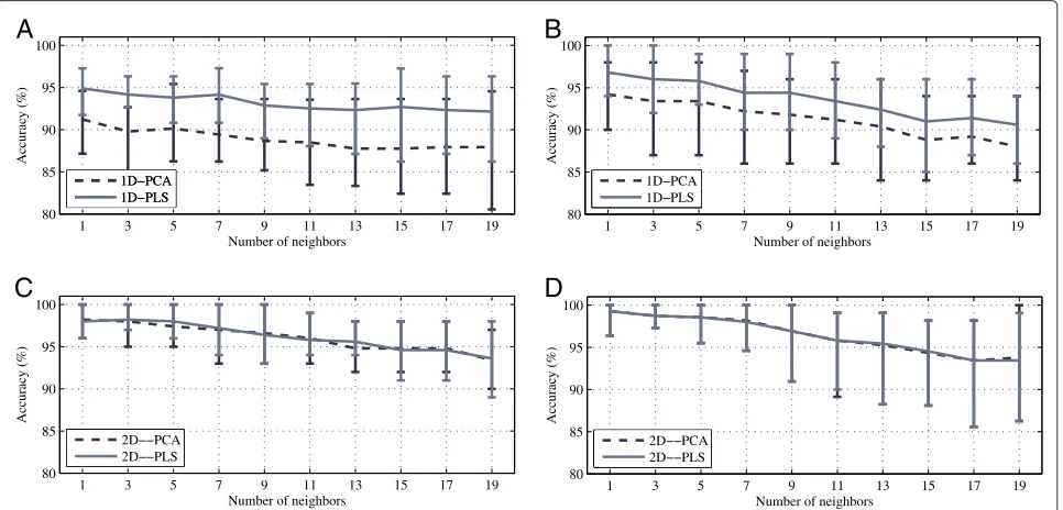
By stepwise increasing the number of neighbors, kˇ, the optimal value was determined as the one which pro-vided the highest accuracy. The procedure was done for each algorithm, by using all thet–f representations avail-able in each scenario, and the relevance threshold was selected as η = 100% (i.e., no relevance criterion was introduced). Additionally, the number of components for PCA/PLS (nfor the 1D methods, nr and nc for the 2D methods) were selected based on the number of com-ponents that describes the 90% of the total variability of the dataset.

Figures 5A,B show the accuracy using the point selection methods described in Algorithm 1, while Figures 5C,D show the results for the methods based on the selection of frequency bands described in Algorithm 2. In the framework of the scenario 1, Figure 5A shows that applying Algorithm 2 to the PCG data, the accu-racy of the classifier decreases as the number of neigh-bors increases. Moreover, the standard deviation is lower for intermediate values and becomes larger as the num-ber of neighbors increases. In the context of the sce-nario 2, Figure 5B shows similar conclusions for EEG signals.

Similar trends appear using the method based on the selection of frequency bands (Algorithm 2). Figures 5C,D show that the performance decreases as the number of neighbors increases for the PCG and EEG databases

1 3 5 7 9 11 13 15 17 19 80

85 90 95 100

Accuracy (%)

Number of neighbors

1 3 5 7 9 11 13 15 17 19 80

85 90 95 100

Accuracy (%)

Number of neighbors

1 3 5 7 9 11 13 15 17 19 80

85 90 95 100

Accuracy (%)

Number of neighbors

1 3 5 7 9 11 13 15 17 19 80

85 90 95 100

Accuracy (%)

Number of neighbors

A

B

C

D

1D−PCA 1D−PLS

2D−−PCA 2D−−PLS 1D−PCA 1D−PLS

1D−PCA 1D−PLS

2D−−PCA 2D−−PLS

(scenarios 1 and 2). Note that the results using Algorithm 2 are more stable than with Algorithm 1. These results reflect the overall structure of the feature spaces obtained.

Accordingly, for both Algorithms, the optimal number of neighbors was fixed askˇ = 1 for the PCG database, and kˇ = 3 for the EEG database. After the feature selection stage, the decision boundary among classes is expected to be clearer than when no relevance measures are used. Thus, after the relevance analysis, the number of neighborskˇof the classifier could be tuned in a higher value, however, the initial estimation (no relevance) is an admissible approximation.

Selection of the relevant features

The variable selection was carried out choosing the most relevant features according to the proposed measures of relevance: linear correlation,ρlc, and symmetrical uncer-tainty, ρsu. The training sets of the t–f representations for the PCG and EEG signals were used to compute

point–wise relevance measures, yielding to a relevance matrix, which is a dependence measure of eacht–f point with its respective label. As a result, a global measure of the degree of dependence is accomplished. Therefore, the amount of features is selected according to a uni-versal threshold fixed a priori over the relevance map, which shows thet–f areas or frequency bands with higher relation to the phenomena under study. Additionally, as explained above, the threshold is varied as a function of the total number of features in hand, i.e., the higher the number of selected features, the lower the relevance threshold.

Figure 6 shows the results of each relevance mea-sure for the scenarios 1 and 2. In particular, the rel-evance measures, shown in Figures 6A,B for the PCG database (scenario 1), demonstrate that a large span of the time–frequency range is poorly relevant. Only some small areas that are clearly defined can be regarded as highly relevant. The relevance measures based on linear cor-relation and symmetrical uncertainty select those time instants in the systole and diastole, where normal heart

0 0.5 0 0.5 1 1.5 2

Frequency [kHz]

ρ_rF su

Time [s]

0 0.2 0.4 0.6 0.8 1 1.2

0 20 40 60 80 100 0

0.5 1

Percentage of features

ρsu

0 0.5 0 0.5 1 1.5 2

Frequency [kHz]

ρ_rF lc

Time [s]

0 0.2 0.4 0.6 0.8 1 1.2

0 20 40 60 80 100 0

0.5 1

Percentage of features

ρlc

0 0.5 1 20 40 60 80

Frequency [Hz]

ρ_rF lc

Time [s]

0 5 10 15 20

0 20 40 60 80 100 0

0.5 1

Percentage of features

ρlc

0 0.5 1 20 40 60 80

Frequency [Hz]

ρ_rF su

Time [s]

0 5 10 15 20

0 20 40 60 80 100 0

0.5 1

Percentage of features

ρsu

A

B

C

D

murmurs should be present. Regarding the EEG database, in the context of the scenario 2, Figures 6C,D demonstrate that the most relevant zones are in the low frequency bands (0–40 Hz). This result is more comprehensible for the symmetrical uncertainty relevance measure, and stands in the fact that epilepsy is directly related with low frequency components [5].

In order to find the most relevant features, the relevance measures estimated were reshaped as vectors and later sorted from highest to lowest values. For both databases, the relevance vectors sorted using the relevance measures considered are shown at the bottom of each subfigure in Figure 6. In the case of the t–f point selection, and using the methodology described in Algorithm 1, the vari-ables were selected according to their relevance, select-ing those with a value over a certain threshold η. Such threshold should be adjusted to optimize the accuracy of the classifier.

Regarding to the selection of the frequency bands described in Algorithm 2, the relevance measures were averaged over the time axis. As a result, a vector corre-sponding to the relevance of the frequency axis is calcu-lated. The values of relevance,ρ_rF

lcandρrFsu, correspond-ing to the frequency axis for both databases are shown in the left plots of each subfigure in Figure 6. Thus, the fre-quency bands were selected according to their relevance.

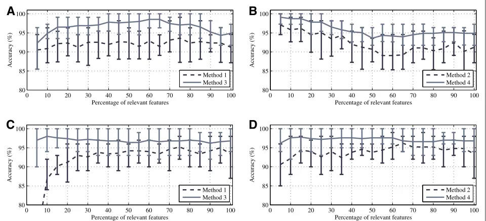
In order to assess the effectiveness of each relevance measure, and using the accuracy of the classifier as a figure of merit, the number of relevant features selected was increased as a percentage of the total number of variables. The percentages were varied from 5 to 100% with steps of 5%. This test was carried out for both

relevance measures (linear correlation and symmetri-cal uncertainty), both methods of dimensionality reduc-tion (PCA and PLS), and for scenarios 1 and 2 (PCG: Figures 7A,B; EEG: Figures 7C,D) using Algorithm 1. For both scenarios, the most stable measure is based on the symmetrical uncertainty, demonstrating that it is possible to accurately classify the PCG and EEG signals using around the 15% of the information given by each

t–f representation.

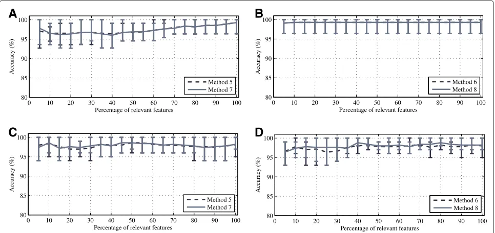
A similar test was carried out for the Algorithm 2, varying the threshold of the relevance of the frequency axis and selecting the most relevant frequency bands. The percentages were varied from 5 to 100% with steps of 5%. The results are shown in Figure 8: Figures 8A,B correspond to the scenario 1, whereas Figures 8C,D cor-respond to the scenario 2. For both scenarios, there is a small and constant performance drop as the number of relevant features diminishes. Once again, symmetri-cal uncertainty provided more stable and selective results, giving high accuracy rates using a very small portion of the

t–f representation.

Data transformation by linear decomposition methods After selecting the most relevant variables, the data set obtained (comprising the most relevant variables) was further reduced using the linear transformation methods commented before. The amount of latent componentsn

for 1D–PCA (methods 1 and 2) and 1D–PLS (methods 3 and 4), as well as the number of timenc and frequency nr components for 2D–PCA (methods 5 and 6) and 2D– PLS (methods 7 and 8), was selected according to the maximum classification rate obtained.

0 10 20 30 40 50 60 70 80 90 100 80

85 90 95 100

Accuracy (%)

Percentage of relevant features

Method 1 Method 3

0 10 20 30 40 50 60 70 80 90 100 80

85 90 95 100

Accuracy (%)

Percentage of relevant features

Method 2 Method 4

0 10 20 30 40 50 60 70 80 90 100 80

85 90 95 100

Accuracy (%)

Percentage of relevant features

Method 1 Method 3

0 10 20 30 40 50 60 70 80 90 100 80

85 90 95 100

Accuracy (%)

Percentage of relevant features

Method 2 Method 4

A

B

C

D

0 10 20 30 40 50 60 70 80 90 100 80

85 90 95 100

Accuracy (%)

Percentage of relevant features

Method 5 Method 7

0 10 20 30 40 50 60 70 80 90 100 80

85 90 95 100

Accuracy (%)

Percentage of relevant features

Method 6 Method 8

0 10 20 30 40 50 60 70 80 90 100 80

85 90 95 100

Accuracy (%)

Percentage of relevant features

Method 5 Method 7

0 10 20 30 40 50 60 70 80 90 100 80

85 90 95 100

Accuracy (%)

Percentage of relevant features

Method 6 Method 8

A

B

C

D

Figure 8Tuning relevant features 2D.Classifier accuracy versus number of relevant variables for 2D methods.(A),(B): scenario 1;(C),(D): scenario 2.

For the point–wise approach given in Algorithm 1, Figures 9A,D illustrate the classifier accuracy when the number of components of the linear decomposition meth-ods (PCA and PLS) changes. In the framework of the scenario 1, for the case of PCG signals, Figure 9A shows that using PCA, a good accuracy is achieved with a num-ber of components over n = 12, whereas n = 21 for PLS. In the context of the scenario 2, for the EEG signals, the results shown in Figure 9D demonstrate that, in both approaches, the performance tends to be steady for a rel-atively small number of components aroundn = 13, for PLS, andn=25 for PCA.

Figures 9B,C,E,F show the performance of the clas-sifier vs. the number of column and row components of the 2D methods used in Algorithm 2. Figures 9B,E show the classifier outcomes using the 2D–PCA methods, while Figures 9C,D show the results using the 2D–PLS methods proposed.

In the scenario 1, the number of row and column com-ponents of thet–f representation of PCG signals must be augmented to achieve a stable behavior. In the case of EEG signals used in the scenario 2, both methods provided a stable behavior as the number of components in rows and columns increased. Furthermore, the accuracy increased with a small number of column components, whereas it got stable as the number of row components augmented. Since the column components are related to the temporal activity, and the row components are associated with the spectral variability, the behavior exhibited by the EEG sig-nals can be interpreted as a smooth temporal activity with

a higher spectral variability, while in PCG both temporal and spectral activities present a large variability.

Summary of results

0 5 10 15 20 25 30 80

85 90 95 100

Accuracy (%)

Number of components

0 5 10 15 20 25 30 80

85 90 95 100

Accuracy (%)

Number of components

0 5 10 15 20 25 30 80

85 90 95 100

Accuracy (%)

Number of components

0 5 10 15 20 25 30 80

85 90 95 100

Accuracy (%)

Number of components

0 5 10 15 20 25 30 80

85 90 95 100

Accuracy (%)

Number of components

0 5 10 15 20 25 30 80

85 90 95 100

Accuracy (%)

Number of components

A

B

C

D

E

F

1D−PCA 1D−PLS

Rows Cols

Rows Cols

1D−PCA 1D−PLS

Rows Cols

Rows Cols

Figure 9Tuning number of components.Accuracy of the classifier versus number of components for the methods considered.(A),(B),(C): scenario 1;(D),(E),(F): scenario 2.

number of splits in both time and frequency axes was fixed empirically.

Finally, the scenario 3 was tested for the methods 4 and 5, since they demonstrated to be the best approaches under study. This scenario presents a more complex clas-sification task involving five different classes. The results obtained are summarized in Table 5 in comparison with the approach found in [5].

Discussion

Several tests were carried out to assess the behavior of the proposed methodologies described in Algorithms 1 and 2. Two different kinds of signals with different stochastic behaviors were tested: PCG signals, with a well defined temporal structure and well localized events; and EEG signals, whose stochastic structure is unfixed. The rele-vance measures clearly reflected the particular stochastic behavior of each kind of signal.

Figure 6 demonstrates that, for EEG signals, the information content is distributed along the time axis, whereas it is well localized in the case of PCG signals. The relevance analysis also demonstrates the presence of

informative and non informative frequency bands. The selectivity of each relevance measure is different and also depends on the specific signal, as it is shown in Figure 6.

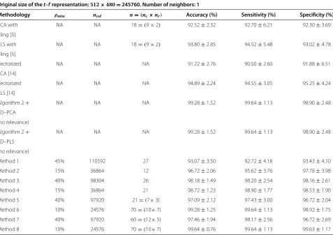
Table 3 Best performance obtained for the methodologies studied using the PCG database (scenario 1)

Original size of thet–frepresentation:512×480=245760. Number of neighbors: 1

Methodology ρmin nrel n=(nc×nr) Accuracy (%) Sensitivity (%) Specificity (%)

PCA with NA NA 18=(9×2) 92.52±2.32 92.70±6.21 92.30±3.69

tiling [5]

PLS with NA NA 18=(9×2) 93.80±2.85 94.52±5.48 93.02±4.78

tiling [5]

Vectorized NA NA NA 91.22±2.76 90.50±2.60 91.88±6.51

PCA [14]

Vectorized NA NA NA 94.89±2.24 94.55±3.05 95.25±4.24

PLS [14]

Algorithm 2+ NA NA NA 99.28±1.52 99.64±1.13 98.90±2.48

2D–PCA

(no relevance)

Algorithm 2₊ NA NA NA 99.28_±1.52 99.64_±1.13 98.90_±2.48

2D–PLS

(no relevance)

Method 1 45% 110592 27 93.07±3.50 92.72±4.18 93.43±4.10

Method 2 15% 36864 12 96.72±2.06 95.62±3.76 97.78±3.98

Method 3 40% 98304 26 98.18±1.49 98.20±2.54 98.16±2.61

Method 4 15% 36864 21 98.72±1.23 98.90±1.77 98.53±1.90

Method 5 40% 97920 21=(7×3) 97.09±2.12 97.43±3.00 96.72±2.04

Method 6 10% 24576 70=(10×7) 99.28±1.25 99.64±1.13 98.92±1.75

Method 7 40% 97920 60=(12×5) 97.46±1.94 98.17±2.56 96.72±2.69

Method 8 10% 24576 70=(10×7) 99.64±0.76 99.64±1.13 99.63±1.17

according to the previous results using the Algorithms 1 and 2, the best relevance measure is the symmetrical uncertainty, given its selectivity and effectiveness for provided feature selection, and its stability in the accuracy. In the scenario 2, for EEG signals, the behavior for both relevance measures is quite similar. The relevance measure based on the symmetrical uncertainty is the most selective, which is reflected in a more sustained accuracy rate (Figure 7D), compared with the fast dec-lination of the performance shown in Figure 7C, where the linear correlation relevance measure is considered. Regarding to the 2D methods, the linear correlation and the symmetrical uncertainty showed the highest values of relevance for the lower frequency bands. Regarding the linear decomposition methods, 1D-PLS and 2D-PLS methods demonstrate, in general, the best performance, exhibiting a difference with respect to PCA around 2 or 3 points of accuracy. However, PCA tends to stabilize the performance of the classifier with a lower quantity of com-ponents, both in the 1D and 2D versions. In any case, the performance of the 1D-PLS and 2D-PLS methods converges with a few amount of components and remains stable.

For the scenario 2, using the 1D methodology (meth-ods 1 to 4), the EEG data needed a small amount of features to achieve high performance rates. Also, the num-ber of temporal components of the 2D methodology is very low, which means that the stochastic activity is eas-ier to parameterize using the 2D approaches. On the other hand, PCG signals need more components in both 1D and 2D approaches, given that local events and specific stochastic behaviors that these signals exhibit must be modeled.

Table 4 Results for the EEG database (scenario 2)

Original size of thet–frepresentation:512×500=256000.Number of neighbors: 3

Methodology ρmin nrel n=(nc×nr) Accuracy (%) Sensitivity (%) Specificity (%)

PCA with NA NA 15=(3×5) 94.00±3.65 (ZO) 94.50±4.38 95.67±4.17

Tiling [5] (NF) 98.50±2.42 95.67±3.17

(S) 84.00±10.75 99.00±1.29

PLS with NA NA 15=(3×5) 93.60±3.37 (ZO) 94.00±4.59 95.67±4.17

Tiling [5] (NF) 98.50±2.42 95.33±2.81

(S) 83.00±10.59 98.75±1.32

Vectorized NA NA NA 93.40±4.12 (ZO) 97.00±4.22 94.00±2.63

PCA [14] (NF) 93.50±4.12 97.00±3.31

(S) 86.00±16.47 98.50±2.11

Vectorized NA NA NA 96.00±2.98 (ZO) 100.00±0.00 95.33±3.58

PLS [14] (NF) 95.50±4.97 98.00±2.81

(S) 89.00±11.01 100.00±0.00

Algorithm 2₊ NA NA NA 98.00_±1.88 (ZO) 100.00±0.00 98.66±2.33

2D–PCA (NF) 99.00±2.10 98.00±2.33

(no relevance) (S) 92.00±7.88 100.00±0.00

Algorithm 2+ NA NA NA 98.20±1.13 (ZO) 100.00±0.00 98.33±2.35

2D–PLS (NF) 99.00±2.10 98.66±1.72

(no relevance) (S) 93.00±4.83 100.00±0.00

Method 1 50% 128000 20 94.40±2.95 (ZO) 99.00±2.11 94.00±4.10

(NF) 91.50±6.69 97.00±4.29

(S) 91.00±11.97 99.75±0.79

Method 2 15% 38400 25 94.80±3.29 (ZO) 95.00±4.71 95.00±4.23

(NF) 95.00±3.33 97.33±2.63

(S) 94.00±8.43 99.25±1.21

Method 3 15% 38400 9 97.80_±1.14 (ZO) 98.00±2.58 99.33±1.41

(NF) 98.00±2.58 98.00±1.72

(S) 97.00±4.83 99.25±1.21

Method 4 10% 25600 13 98.20±1.99 (ZO) 98.50±2.42 99.00±2.25

(NF) 98.50±3.37 98.00±1.72

(S) 97.00±4.83 100.00±0.00

Method 5 50% 128000 425=(17×25) 98.80±1.03 (ZO) 100.00±0.00 99.00±1.61

(NF) 99.00±2.11 99.33±1.49

(S) 96.00±5.16 99.75±0.79

Method 6 45% 115200 442=(17×26) 98.40±1.26 (ZO) 100.00±0.00 99.33±1.41

(NF) 99.00±2.11 98.33±2.36

(S) 94.00±6.99 99.75±0.79

Method 7 45% 115200 42=(3×14) 98.60±0.97 (ZO) 100.00±0.00 99.00±1.61

(NF) 98.00±2.58 99.33±1.41

(S) 97.00±4.83 99.50±1.05

Method 8 40% 102400 784=(28_×28) 98.80_±1.03 (ZO) 100.00±0.00 99.33±1.41

(NF) 99.50±1.58 98.67±1.72

(S) 95.00±5.27 100.00±0.00

Table 5 Results for the five class problem with the EEG database (scenario 3)

Methodology Accuracy (%) Sensitivity (%) Specificity (%)

Tiling + PLS [5] 79.40_±7.00 Z 71.00_±16.33 93.00_±3.07

O 83.00±11.60 94.75±3.81

N 85.00±13.54 92.25±4.16

F 73.00±14.94 95.00±3.54

S 85.00±8.50 99.25±1.21

Method 4 91.00±1.94 Z 93.00±6.75 97.00±2.58

O 94.00±6.99 99.25±1.21

N 94.00±5.16 95.00±2.64

F 77.00±9.49 98.00±2.30

S 97.00±4.83 99.50±1.05

Method 8 94.40±3.75 Z 99.00±3.16 98.25±2.06

O 95.00_±7.07 99.50_±1.58

N 96.00_±5.16 97.00_±1.58

F 88.00_±10.33 98.50_±1.75

S 94.00_±6.99 99.75_±0.79

of the process, because the size of the matrices is further reduced before the dimensionality reduction process.

Regarding the scenario 3, the results obtained with methods 4 and 8 outperformed those using the algorithm in [5] (up to 10 classification points). Nevertheless, the band selection methodology described in Algorithm 2 (method 8) is more suitable to discriminate among the different classes.

The values that gave the best accuracy rates for each database and for each methodology (1D and 2D) are sum-marized in Table 6 (methods 4 and 8). The percentage of reduction is computed as the ratio of features removed with the total number of features. This measure is com-puted for the first stage of variable selection by relevance analysis (% Reduc. 1) as well as for the second stage of linear transformation by PCA or PLS (% Reduc. 2).

The feature selection stage allows an effective selec-tion of the most relevant features. In accordance with the results shown in Table 6 for the scenario 1, an accuracy

of 99.64% was obtained with only 10% of the features extracted from the PCG signals; and for the EEG database, accuracies of 98.80 and 94.40% were obtained for the scenarios 2 and 3, respectively, by using 40% of thet–f

features.

On the other hand, the methodology of Algorithm 1 needed a lower quantity of components, which is reflected in a lower feature space dimensionality; but Algorithm 2 allows larger matrices with almost the same performance. In the case of the 1D methodology (methods 1 to 4), and for data matrices of size(F·T)×K, it is necessary to com-pute transformation matrices of size(F·F)×n, while for the 2D methodology (methods 5 to 8), two transformation matrices ofF×nrandT×ncare needed while working with two data matrices of sizeT×(F·K)andF×(T·K).

Conclusions

This research proposes a new and promising approach for feature selection over t–f based features that can be applied to non-stationary biosignal classification. The results obtained showed a high performance under differ-ent scenarios and demonstrated that the accuracy is stable for EEG and PCG signals, giving evidence of the general-ization capabilities of the proposed methodology for dif-ferent signals with diverse non-stationary behaviors. The results open the possibility to extrapolate the methodol-ogy to the study of other biosignals.

The method directly deals with highly redundant and irrelevant data contained in the bi-dimensionalt–f rep-resentations, combining a first stage of irrelevant data removal by variable selection using a relevance measure, with a second stage of redundancy reduction by lin-ear transformation methods. Under these premises, two methodologies have been derived: the first one aimed to find the most relevant t–f points; the second one devised to select the frequency bands with a higher relevance. Each methodology needs a particular linear decomposition approach: in the first case, PCA and PLS methods were used, whereas, in the second approach, a to the matrix-data based generalization these methods was used.

Table 6 Summary of best performance rates for each database

Methodology t–f nrel % Reduc. 1 n=(nc×nr) % Reduc. 2 Accuracy

representation

size

PCG - Method 4 245760, 36864 85% 21 94.30% 98.20_±1.99%

Scenario 1 Method 8 (512_×480) 24576 90% 70₌(10_×7) 71.52% 99.64_±0.66%

EEG - Method 4 256000, 25600 90% 13 99.99% 98.20±1.99%

Scenario 2 Method 8 (512×500) 102400 60% 784=(28×28) 70% 98.72±1.23%

EEG - Method 4 256000, 25600 90% 13 99.99% 91.00±1.94%

Although this work uses the spectrograms, the pro-posed approaches can be applied to other kind of real-valued t–f representations, such as time-frequency distributions, wavelet transforms, and matching pursuit, among others.

The relevance analysis was evaluated using two super-vised measures: linear correlation and symmetrical uncer-tainty. Under the same premises, the application of these measures demonstrated a significant improvement in comparison with the case when no relevance measure was used. Besides, the relevance measure based on the symmetrical uncertainty provided a better performance, allowing an effective selection of the most relevant vari-ables, thus diminishing the computational burden of the linear decomposition methods and of the classifier. In addition, the relevance analysis serves itself as an interpre-tation tool, giving information about those t–f patterns closer related to abnormalities and pathological behavior.

On the other hand, it was found that the use of a super-vised method (such as PLS) clearly improved the perfor-mance of the classifier. Moreover, the perforperfor-mance of the 1D and 2D versions was found almost similar. Although the 1D methodology needs a lower quantity of compo-nents, which is reflected in a lower feature space dimen-sionality, the 2D methodology allows to take into account the dynamic information of each spectral component over thet–f planes, which was reflected in more stable results. As a future study, the introduction of the relevance measure directly into the linear decomposition method should be evaluated; so a relevance and a redundancy analysis could be carried out in the same step, but prob-ably at the expense of a larger computational burden and memory requirements. Additionally, the use of other linear or nonlinear decomposition techniques, such as linear discriminant analysis or local linear embedding should be evaluated. Moreover, the use of other rele-vance measures such as mutual information might also be considered, since it is an effective criterion for feature selection algorithms.

Competing interests

The authors declare that they have no competing interest.

Acknowledgements

This research was supported by “Centro de Investigaci´on e Innovaci´on de Excelencia - ARTICA,Programa Nacional de Formaci´on de Investigadores ”GENERACI ´ON DEL BICENTENARIO”, 2011,” funded by COLCIENCIAS, “Servicio de monitoreo remoto de actividad cardiaca para el tamizaje clinico en la red de telemedicina del departamento de Caldas” funded by Universidad Nacional de Colombia and Universidad de Caldas and through the project grant TEC2009-14123-C04-02 financed by the Spanish government.

Author details

1_{Signal Processing and Recognition Group, Universidad Nacional de} Colombia, Km. 9, Va al Aeropuerto, Campus la Nubia, Caldas, Manizales, Colombia.2_{Departamento de Ingeniera de Circuitos y Sistemas, Universidad} Politcnica de Madrid, Ctra. de Valencia, km. 7, 28031 Madrid, Spain.

Received: 1 December 2011 Accepted: 28 August 2012 Published: 9 October 2012

References

1. LM Sepulveda-Cano, CD Acosta-Medina, G Castellanos-Dominguez, Relevance Analysis of Stochastic Biosignals for Identification of Pathologies. EURASIP J. Adv. Signal Process.2011, 10 (2011)

2. E Sejdic, I Djurovic, J Jiang, Time-frequency feature representation using energy concentration: an overview of recent advances. Digital Signal Process.19, 153–183 (2009)

3. L Avendano-Valencia, J Godino-Llorente, M Blanco-Velasco, G Castellanos-Dominguez, Feature extraction from parametric time-frequency representations for heart murmur detection. Annals Biomed. Eng.38(8), 2716–2732 (2010)

4. MP Tarvainen, S Georgiadis, JA Lipponen, M Hakkarainen, PA Karjalainen. Time-varying spectrum estimation of heart rate variability signals with Kalman smoother algorithm, (2009), pp. 1–4

5. A Tzallas, M Tsipouras, D Fotiadis, Epileptic seizure detection in electroencephalograms using time-frequency analysis. IEEE Trans. Inf. Technol. Biomed.13(5), 703–710 (2009)

6. AF Quiceno-Manrique, JI Godino-Llorente, M Blanco-Velasco, G Castellanos-Dominguez, Selection of dynamic features based on time-frequency representations for heart murmur detection from phonocardiographic signals. Annals Biomed. Eng.38, 118–37 (2010) 7. S Debbal, F Bereksi-Reguid, Time–frequency analysis of the first and the

second heartbeat sounds. Appl. Math. Comput.128(2), 1041–1052 (2007) 8. S Jabbari, H Ghassemian, Modeling of heart systiloc murmurs based on

multivariate matching pursuit for diagnosis of valvular disorders. Comput. Biol. Med.41, 802–811 (2011)

9. PJ Durka, A Matysiak, E Mart´ınez-Montes, P Valdes-Sosa, KJ Blinowska, Multichannel matching pursuit and EEG inverse solutions. J. Neurosci. Methods.148, 49–59 (2005)

10. AS Zandi, M Javidan, GA Dumont, RT Freshi, Automated real-ti me epileptic seizure detection in scalp eeg recordings using a n algorithm based on wavelet packet transform. IEEE Trans. Biomed. Eng.57(7), 1639–1651 (2010)

11. D Cvetkovic, ED ¨Ubeyli, I Cosic, Wavelet transform feature extraction from human PPG , ECG , and EEG signal responses to ELF PEMF exposures: a pilot study. Digital Signal Process.18(5), 861–874 (2008)

12. B Gillespie, L Atlas, Optimizing time-frequency kernels for classification. IEEE Trans. Signal Process.49(3), 485–496 (2001)

13. S Haufe, R Tomioka, T Dickhaus, C Sannelli, B Blankertz, G Nolte, KR M ¨uller, Large-scale EEG/MEG source localization with spatial flexibility. NeuroImage.54, 851–859 (2011)

14. E Bernat, W Williams, W Gehring, Decomposing ERP time–frequency energy using PCA. Clin. Neurophys.116, 1314–1334 (2005)

15. E Grall-Maes, P Beauseroy, Mutual information-based feature extraction on the time-frequency plane. IEEE Trans. Signal Process.50(4), 779–790 (2002) 16. Y Zhao, S Zhang, Generalized dimension-reduction framework for

recent-biased time series analysis. IEEE Trans. Knowl. Data Eng.18(2), 231–244 (2006)

17. M Barker, W Rayens, Partial least squares for discrimination. J. Chemomet. 17(3), 166–173 (2003)

18. J Yang, D Zhang, A Frangi, J Yang, Two-dimensional PCA: a new approach to appearance-based face representation and recognition. IEEE Trans. Pattern Anal. Mach. Intell.26, 131–137 (2004)

19. D Zhang, ZH Zhou, (2D)2PCA: two-directional two-dimensional PCA for efficient face representation and recognition. Neurocomputing.69(1–3), 224–231 (2005)

20. L Yu, H Liu, Efficient feature selection via analysis of relevance and redundancy. J. Mach. Learn. Res.5, 1205–1224 (2004)

21. R Andrzejak, K Lehnertz, C Rieke, F Mormann, P David, C Elger, Indications of nonlinear deterministic and finite dimensional structures in time series of brain electrical activity: Dependence on recording region and brain state. Phys. Rev. E.64, 71–86 (2001)

22. R Duda, P Hart,D Stork Pattern Classification 2nd edn. with Computer Manual 2nd Edition Set(Wiley, 2001)

doi:10.1186/1687-6180-2012-219