Sequential Genetic Search for Ensemble Feature Selection

Sequential Genetic Search for Ensemble Feature Selection

Alexey Tsymbal

Mykola Pechenizkiy Pádraig

Cunningham

Dept. of Computer Science Dept. of CS & ISs Dept. of Computer Science

Trinity

College

Dublin

University

of

Jyväskylä Trinity

College

Dublin

Dublin 2, Ireland P.O. Box 35, Finland-40351 Dublin 2, Ireland

[email protected]

[email protected] [email protected]

Abstract

Ensemble learning constitutes one of the main di-rections in machine learning and data mining. En-sembles allow us to achieve higher accuracy, which is often not achievable with single models. One technique, which proved to be effective for con-structing an ensemble of diverse classifiers, is the use of feature subsets. Among different approaches to ensemble feature selection, genetic search was shown to perform best in many domains. In this paper, a new strategy GAS-SEFS, Genetic Algo-rithm-based Sequential Search for Ensemble Fea-ture Selection, is introduced. Instead of one genetic process, it employs a series of processes, the goal of each of which is to build one base classifier. Ex-periments on 21 data sets are conducted, comparing the new strategy with a previously considered ge-netic strategy for different ensemble sizes and for five different ensemble integration methods. The experiments show that GAS-SEFS, although being more time-consuming, often builds better ensem-bles, especially on data sets with larger numbers of features.

1 Introduction

A popular method for creating an accurate model from a set of training data is to construct a set (ensemble) of classifiers. It was shown that an ensemble is often more accurate than any of the single classifiers in it. The integration of classifi-ers is currently an active research area in the machine learn-ing and neural networks communities [Dietterich, 1997].

Both theoretical and empirical research have demon-strated that a good ensemble should include diverse base classifiers. Another important issue in creating an effective ensemble is the choice of the function for combining the predictions of the base classifiers. It was shown that increas-ing the ensemble diversity is not enough to ensure increased accuracy – if the integration method does not properly util-ize the ensemble diversity, then no benefit arises from the integration [Brodley and Lane, 1996].

One effective approach for generating an ensemble of di-verse classifiers is the use of feature subsets, or ensemble feature selection [Opitz, 1999]. By varying the feature

sub-sets used to generate the base classifiers, it is possible to promote diversity and produce base classifiers that tend to err in different sub-areas of the instance space.

Feature selection algorithms, including ensemble feature selection, are typically composed of the following compo-nents [Aha and Bankert, 1995, Opitz, 1999]: (1) search strategy, that searches through the space of feature subsets;

and (2) fitness function, that inputs a feature subset and

out-puts a numeric evaluation. The search strategy’s goal is to find a feature subset maximizing this function.

It is reasonable to include in the fitness function, explic-itly or implicexplic-itly, both accuracy and diversity. One measure of fitness, which was proposed in [Opitz, 1999], defines fitness Fitnessi of classifier i corresponding to feature subset

i to be proportional to classification accuracy acci and

diver-sity divi of the classifier:

i i

i acc div Fitness = +α⋅ , (1)

where α reflects the influence of diversity. Diversity divi is

the contribution of classifier i to the total ensemble

sity, which can be measured as the average pairwise diver-sity for all the pairs of classifiers including i. This fitness

function was also used in experiments in [Tsymbal et al.,

2003; 2005], and it is used in the experiments in this paper. In [Tsymbal et al., 2005] a genetic search-based strategy

GA has been introduced. It uses genetic search for evolving the initial population built with random subspacing. GA was shown to perform best on average with respect to the other three strategies, and two diversity measures were best for GA of the five considered measures: the kappa statistic, and the fail/non-fail disagreement.

In this paper, we introduce a new genetic search-based strategy for ensemble feature selection, GAS-SEFS, which, instead of maintaining a set of feature subsets in each gen-eration like in GA, consists in applying a series of genetic processes, one for each base classifier, sequentially.

2 Ensemble Feature Selection and Random

Subspacing

The task of using an ensemble of models can be broken down into two basic questions: (1) what set of models should be generated?; and (2) how should the predictions of the models be integrated? [Dietterich, 1997].

One effective approach to ensemble generation is the use of different subsets of features for each model. Finding a set of feature subsets for constructing an ensemble is also known as ensemble feature selection [Opitz, 1999]. While

traditional feature selection algorithms have the goal of finding the best feature subset that is suitable to both the learning problem and the learning algorithm, the task of ensemble feature selection has the additional goal of finding a set of feature subsets that will promote diversity among the base classifiers [Opitz, 1999].

Ho [1998] has shown that simple random selection of fea-tures may be an effective technique for ensemble feature selection because the lack of accuracy in the ensemble members is compensated for by their diversity. This tech-nique is called the random subspace method or simply Ran-dom Subspacing (RS).

With RS one may solve the small sample size problem, because the training sample size relatively increases in ran-dom subspaces. Ho [1998] shows that while most other classification methods suffer from the curse of dimensional-ity, this method does not. RS has much in common with bagging [Skurichina and Duin, 2001], but instead of sam-pling instances, one samples features. Like bagging, RS is a parallel learning algorithm, that is, generation of each base classifier is independent. This makes it suitable for parallel implementation that is desirable in some practical applica-tions. It was shown that, like in bagging, accuracy could be only increased with the addition of new members, even when the ensemble complexity grew [Ho, 1998].

RS is used as a base in a number of ensemble feature se-lection strategies, e.g. GEFS (Genetic Ensemble Feature Selection) [Opitz, 1999] and HC (Hill Climbing) [Cunning-ham and Carney, 2000].

3 Two Strategies for Genetic Ensemble

Fea-ture Selection

3.1 GA and GAS-SEFS

The use of genetic search has been an important direction in the feature selection research. Genetic algorithms have been shown to be effective global optimization techniques. The use of genetic algorithms for ensemble feature selection was first proposed in [Kuncheva, 1993] and further elaborated in [Kuncheva and Jain, 2000]. As the fitness function in [Kuncheva, 1993; Kuncheva and Jain, 2000] the ensemble accuracy was used instead of the accuracy of the base classi-fiers. However, such a fitness function is biased towards some particular integration method (often simple voting). Besides, as it was shown e.g. in [Kuncheva, 1993], such a design is prone to overfitting, and some additional preven-tive measures are needed to be taken to avoid this (as

in-cluding in the fitness function penalty terms accounting for the number of features). The use of individual accuracy and diversity as in (1) is an alternative solution to this problem. Another motivation for this alternative is the fact that over-fitting at the level of the base classifiers is more desirable than overfitting of the ensemble itself. It was shown recently in several studies that an ensemble of overfitted members might often be better than an ensemble of non-overfitted members. For example, in [Street and Kim, 2001] pruning trees resulted in decreased ensemble accuracy, even though the accuracy of the trees themselves increased.

The Genetic Algorithm for ensemble feature selection (GA) [Tsymbal et al., 2005] is based on the GEFS strategy

of Opitz [1999]. GEFS was the first genetic algorithm for ensemble feature selection that explicitly used diversity in its fitness function. GA begins with creating an initial popu-lation with RS. Then, new candidate classifiers are produced by crossover and mutation. After producing a certain num-ber of individuals the process continues with selecting a new subset of candidates randomly with a probability propor-tional to fitness (so called roulette-wheel selection). The process of creating new classifiers and selecting a subset of them (a generation) continues a certain number of times. After a predefined number of generations, the fittest indi-viduals make up the population, which comprises the en-semble. The representation of each individual is a constant-length string of bits, where each bit corresponds to a particu-lar feature. The crossover operator uses uniform crossover, in which each feature of the two children takes randomly a value from one of the parents. The mutation operator ran-domly toggles a number of bits in an individual.

Instead of maintaining a set of feature subsets in each generation of one genetic process, GAS-SEFS (Genetic Al-gorithm-based Sequential Search for Ensemble Feature Se-lection) uses a series of genetic processes, one for each base classifier, sequentially. Pseudo-code for GAS-SEFS is given in Figure 1. After each genetic process one base classifier is selected into the ensemble. GAS-SEFS uses the same fitness function (1), but diversity is calculated with the base classi-fiers already formed by previous genetic processes instead of the members of current population. In the first GA proc-ess, the fitness function has to use accuracy only. GAS-SEFS uses the same genetic operators as GA.

For I=1 to EnsembleSize

For J=1 to 10 Population(J)=RSM(#Features); For J=1 to #Generations

For K=1 to 10 CalculateFitness(Population(K)); For K

(L,M)=Select2(Population); Offsprings(K)=CrossOver(L,M); EndForK

For K=1 to 10 Mutate1_0(Offsprings(20+K)); Mutate0_1(Offsprings(30+K)); For K=1 to 40 CalculateFitness(Offsprings(K));

//randomly proportional to fitness

Population=Select10(Population+Offsprings); EndForJ

//according to fitness

BaseClassifier(I)=Select1(Population); EndForI

GA has a number of peculiarities, which we use also in GAS-SEFS. Full feature sets are not allowed in RS nor may the crossover operator produce a full feature subset. Indi-viduals for crossover are selected randomly proportional to log(1+fitness) instead of just fitness, which adds more

di-versity into the new population. The generation of children identical to their parents is prohibited. To provide a better diversity in the length of feature subsets, two different muta-tion operators are used (Mutate1_0 and Mutate0_1), one of

which always deletes features randomly with a given prob-ability, and the other – adds features.

Parameter settings for our implementation of GA and GAS-SEFS include a mutation rate of 50%, a population size of 10, a search length of 40 feature subsets (the number of new individuals produced by crossover and mutation), of which 20 are offsprings of the current population of 10 clas-sifiers generated by crossover, and 20 are mutated off-springs (10 with each mutation operator). 10 generations of individuals were produced, as our pilot studies have shown that in most cases, with this configuration, the ensemble accuracy does not improve after 10 generations, due to over-fitting the training data.

The complexity of GA does not depend on the number of features, and is , where is the number of individuals in one generation, and gen is the number of generations [Tsymbal et al., 2005]. The complexity of

GAS-SEFS is , where S is the number of base

classifiers. In our experiments, on average, GA and GAS-SEFS look through about 400 and 4000 feature subsets cor-respondingly (given that the number of base classifiers is 10, the number of individuals in a generation is 40, and the number of generations is 10).

) (S N_gen

O ⋅′ S′

N

) (S S N_gen O ⋅ ′⋅

3.2 Diversity measures used in the fitness function

The fail/non-fail disagreement measure and the kappa statis-tic were shown to provide the best performance for GA in [Tsymbal et al., 2005].

The fail/non-fail disagreement measure was defined in

[Skalak, 1996] as the percentage of test instances for which the classifiers make different predictions but for which one of them is correct:

00 01 10 11

10 01

_

N N N N

N N dis

div i,j

+ + +

+

= , (2)

where Nab is the number of instances, classified correctly

(a=1) or incorrectly (a=0) by classifier i, and correctly (b=1)

or incorrectly (b=0) by classifier j. The denominator in (2) is

equal to the total number of instances. The fail/non-fail dis-agreement varies from 0 to 1.

The kappa statistic was first introduced in [Cohen, 1960].

Let Nij be the number of instances, recognized as class i by

the first classifier and as class j by the second one, Ni* is the

number of instances recognized as i by the first classifier,

and N*i is the number of instances recognized as i by the

second classifier. Define then Θ1 and Θ2 as:

N N l

i ii

∑

Θ 1

1 , and

∑

⎟ ⎠ ⎞ ⎜

⎝ ⎛ _⋅ =

Θ l

i N

N N Ni i

1

2 * * , (3)

where l is the number of classes and N is the total number of

instances. Θ1 estimates the probability that the two

classifi-ers agree, and Θ2 is a correction term, which estimates the

probability that the two classifiers agree simply by chance (in the case where each classifier chooses to assign a class label randomly). The pairwise diversity div_kappai,j is

de-fined as follows:

2 2 1

1 _

Θ −

Θ − Θ = i,j

kappa

div . (4)

We normalize this measure to vary from 0 to 1.

4

Integration of an Ensemble of Models

The challenging problem of integration is to decide which of the classifiers to select or how to combine the results pro-duced by the base classifiers. A number of selection and combination approaches have been proposed.

One of the most popular and simplest techniques used to combine the results of the base classifiers, is simple voting (also called majority voting) [Bauer and Kohavi, 1999]. In the voting, the output of each base classifier is considered as a vote for that particular class value. The class value that receives the biggest number of votes is selected as the final classification. Weighted Voting (WV), where each vote has a weight proportional to the estimated generalization per-formance of the corresponding classifier, works usually bet-ter than simple voting [Bauer and Kohavi, 1999].

A number of selection techniques have also been proposed to solve the integration problem. One of the most popular and simplest selection techniques is Cross-Validation Ma-jority (CVM, also called Single Best; we call it simply Static Selection, SS, in our experiments) [Schaffer, 1993]. In CVM, the cross-validation accuracy for each base classi-fier is estimated, and then the classiclassi-fier with the highest accuracy is selected.

The described above approaches are static. They select

one model for the whole data space or combine the models uniformly. In dynamic integration each new instance to be

classified is taken into account. Usually, better results can be achieved if integration is dynamic.

We consider in our experiments three dynamic techniques based on the same local error estimates: Dynamic Selection (DS), Dynamic Voting (DV), and Dynamic Voting with Selection (DVS) [Tsymbal and Puuronen, 2000]. They con-tain two main phases. First, at the learning phase, the local classification errors of each base classifier for each instance of the training set are estimated according to the 1/0 loss function using cross validation. The learning phase finishes with training the base classifiers on the whole training set. The application phase begins with determining k-nearest

After, DS simply selects a classifier with the least pre-dicted local classification error. In DV, each base classifier receives a weight that is proportional to its estimated local accuracy, and the final classification is produced as in WV. In DVS, the base classifiers with the highest local classifica-tion errors are discarded (the classifiers with errors that fall into the upper half of the error interval) and locally weighted voting (DV) is applied to the remaining classifiers.

5 Experimental

Investigations

5.1 Experimental setup

The experiments are conducted on 21 data sets taken from the UCI machine learning repository [Blake et al., 1999].

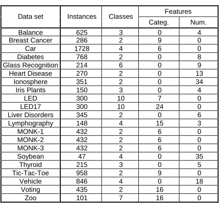
These data sets include real-world and synthetic problems, vary in characteristics, and were previously investigated by other researchers. The main characteristics of the data sets are presented in Table 1.

Table 1 Data sets and their characteristics

Features Data set Instances Classes

Categ. Num. Balance 625 3 0 4 Breast Cancer 286 2 9 0 Car 1728 4 6 0 Diabetes 768 2 0 8 Glass Recognition 214 6 0 9 Heart Disease 270 2 0 13

Ionosphere 351 2 0 34 Iris Plants 150 3 0 4

LED 300 10 7 0 LED17 300 10 24 0 Liver Disorders 345 2 0 6 Lymphography 148 4 15 3 MONK-1 432 2 6 0 MONK-2 432 2 6 0 MONK-3 432 2 6 0 Soybean 47 4 0 35

Thyroid 215 3 0 5 Tic-Tac-Toe 958 2 9 0 Vehicle 846 4 0 18 Voting 435 2 16 0 Zoo 101 7 16 0

As in [Tsymbal et al., 2003; 2005], we use Simple Bayes

(SB) as the base classifier in the ensembles. It has been re-cently shown experimentally and theoretically that SB can be optimal even when the “naïve” feature-independence assumption is violated by a wide margin [Domingos and Pazzani, 1997]. Second, when SB is applied to the sub-problems of lower dimensionalities, the error bias of the Bayesian probability estimates caused by the feature-independence assumption becomes smaller. It also can eas-ily handle missing feature values. Besides, it has advantages in terms of simplicity, learning speed, classification speed, and storage space. We believe that dependencies and con-clusions presented in this paper do not depend on the learn-ing algorithm used and would be similar for most known learning algorithms.

To evaluate GA and GAS-SEFS, we have used stratified random-sampling cross validation with 60 percent of stances in the training set. The remaining 40 percent of

in-stances were divided into two sets of approximately equal size (a validation set and a test set). 70 test runs of were made on each data set for each search strategy and diversity. Four different ensemble sizes have been tested: 3, 5, 7, and 10. The ensemble size did not exceed 10 due to two main reasons: (1) limitation in computational resources, and (2) it was shown in experiments that for guided ensemble construction such as genetic search the biggest gain is achieved already with 10 base classifiers, and much less classifiers are needed than with unguided ensemble con-struction such as RS and bagging.

At each run of the algorithm, accuracies for the five types of ensemble integration are collected: Static Selection (SS), Weighted Voting (WV), Dynamic Selection (DS), Dynamic Voting (DV), and Dynamic Voting with Selection (DVS). We have collected ensemble characteristics for four num-bers of generations: 1, 3, 5, and 10.

To reduce the number of possible combinations of pa-rameters, we conducted a separate series of preliminary ex-periments using the wrapper approach based on cross vali-dation to select the best diversity coefficient α and the number of nearest neighbors in dynamic integration k as in

[Tsymbal et al., 2005]. We have experimented with seven

values of α: 0, 0.25, 0.5, 1, 2, 4, and 8. Seven values: 1, 3, 7, 15, 31, 63, 127 ( ) were used for k. From

the experimental results we could see that the best value of k

depended mostly only on the integration method used and on the data set. The best

7 ,..., 1 , 1 2n− n=

α’s varied with the search strat-egy, integration method, and data set used.

After, the experiments were repeated with the selected values of α and k. Although the same data were used for

the selection and for the later experiments,we believe that this did not lead to overfitting due to the small number of possible values for α and k.

The test environment was implemented within the MLC++ framework (the machine learning library in C++) [Kohavi et al., 1996]. A multiplicative factor of 1 was used

for the Laplace correction in SB as in [Domingos and Paz-zani, 1997]. Numeric features were discretized into ten equal-length intervals (or one per observed value, whichever was less), as it was done in [Domingos and Pazzani, 1997]. Although this approach was found to be slightly less accu-rate than more sophisticated ones, it has the advantage of simplicity, and is sufficient for comparing different ensem-bles of SB classifiers with each other.

5.2 Experimental results

can be seen from the figure that GAS-SEFS builds even more accurate ensembles than GA; especially for group 2 including data sets with larger numbers of features. Accu-racy grows with the ensemble size, but the growth flattens as the number of base classifiers increases.

0.810 0.815 0.820 0.825 0.830 0.835 0.840

GA_gr1 GAS-SEFS_gr1 GA_gr2 GAS-SEFS_gr2 3 5 7 10

Figure 2 Ensemble accuracies for two strategies, two groups of data sets, and four ensemble sizes

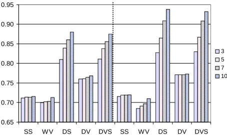
In Figure 3 ensemble accuracies are shown for the two strategies, five integration methods, and four ensemble sizes on the Tic-Tac-Toe data set, as a representative of group 2 including 958 instances and 9 features. This figure supports our previous findings. Besides, it could be seen that dy-namic integration, expectedly, outperforms static integration both for GA and for GAS-SEFS. Accuracy grows with the ensemble size and this growth is greater for the best integra-tion methods (DS and DVS in this case).

0.65 0.70 0.75 0.80 0.85 0.90 0.95

SS W V DS DV DVS SS WV DS DV DVS

3 5 7 10

Figure 3 Ensemble accuracies for GA (left) and GAS-SEFS (right) for five integration methods and four ensemble sizes on the Tic-Tac-Toe data set

The difference between the two strategies is clearer for the best integration methods. The dependencies were the same for all the data sets, with sometimes lesser difference be-tween the integration methods. For some data sets DV out-performs DS, which supports the previous findings about behaviour of the integration methods [Tsymbal and Puu-ronen, 2000; Tsymbal et al., 2005].

5.3 Other interesting findings

Selected values of α were different for different data sets, supporting findings in [Tsymbal et al., 2003; 2005]. In

gen-eral, for both strategies, α for the dynamic integration methods is bigger than for the static ones (2.2 vs 0.8 on av-erage). GAS-SEFS needs slightly higher values of α than GA (1.8 vs 1.5 on average). This can be explained by the fact that GAS-SEFS always starts with a classifier, which is based on accuracy only, and the subsequent classifiers need more diversity than accuracy.

The number of selected features falls as the ensemble size grows, and this is especially clear for GAS-SEFS, as the base classifiers need more diversity. As a rule, more features are needed in the static integration methods than in the dy-namic ones to achieve better accuracy. GAS-SEFS results in slightly smaller feature subsets on average (48% vs 50% of features for dynamic integration strategies).

As it was also reported in [Tsymbal et al., 2005], the

se-lected k-neighbourhood values for dynamic integration

change with the integration method. DS needs higher values of k. This can be explained by the fact that its prediction is

based on only one classifier being selected, and thus, it is very unstable. Higher values of k provide more stability to

DS. The average selected k is equal to 33 for DS, and it is

only 14 for DV. For DVS, as a hybrid strategy, it is in be-tween at 24. The selected values of k do not change

signifi-cantly with the change of the search strategy and the ensem-ble size.

Experimental results for both GA and GAS-SEFS show that the static integration methods, SS and WV, and the dy-namic DS start to overfit the validation set already after 5 generations and show lower accuracies, whereas the accura-cies of DV and DVS continue to grow up to 10 generations. This shows the importance of selection of the appropriate integration method for the genetic strategies.

6 Conclusions

In our paper, we have considered two genetic search strate-gies for ensemble feature selection. The new strategy, GAS-SEFS, consists in employing a series of genetic search proc-esses, one for each base classifier. It was shown in experi-ments that GAS-SEFS results in better ensembles having greater accuracy in many domains, especially for data sets with relatively larger numbers of features. GAS-SEFS is significantly more time-consuming than GA. However, it can be easily parallelized in a multiprocessor setting, and one processor could be used for each offspring in the current generation.

One of the reasons for the success of GAS-SEFS is the fact that each of the core GA processes leads to significant overfitting of a corresponding ensemble member, and, as it was shown before, an ensemble of overfitted members is often better that an ensemble of non-overfitted members.

In [Oliveira et al., 2003] it was shown that besides the use

single feature subset selection is based on Pareto-front dominating solutions. Adaptation of this technique to en-semble feature selection is an interesting topic for further research.

Acknowledgments

This study is supported by Science Foundation Ireland and COMAS Graduate School of the University of Jyväskylä, Finland. We would like to thank the UCI machine learning repository for the data sets, and the MLC++ library for the source code used in this study.

References

[Aha and Bankert, 1995] David W. Aha and Richard L. Bankert. A comparative evaluation of sequential feature selection algorithms. In Proceedings of the 5th Interna-tional Workshop on Artificial Intelligence and Statistics,

pages 1-7, 1995.

[Bauer and Kohavi, 1999] Eric Bauer and Ron Kohavi. An empirical comparison of voting classification algorithms: bagging, boosting, and variants. Machine Learning 36

(1,2): 105-139, 1999.

[Blake et al., 1999] Catherine L. Blake, Eamonn Keogh, and

Chris J. Merz. UCI repository of machine learning data-bases. Dept. of Information and Computer Science,

Uni-versity of California, Irvine, CA, 1999.

[Brodley and Lane, 1996] Carla E. Brodley and Terran Lane. Creating and exploiting coverage and diversity. In

Proceedings of the Workshop on Integrating Multiple Learned Models, pages 8-14, 1996.

[Cohen, 1960] Jacob Cohen. A coefficient of agreement for nominal scales. Educational and Psychological Meas-urement 20, pages 37-46, 1960.

[Cunningham and Carney, 2000] Padraig Cunningham and John Carney. Diversity versus quality in classification ensembles based on feature selection. In Proceedings of the 11th European Conference On Machine Learning,

pages 109-116, Barcelona, Spain, 2000, Springer. [Dietterich, 1997] Tom G. Dietterich. Machine learning

research: four current directions. AI Magazine 18(4):

97-136, 1997.

[Domingos and Pazzani, 1997] Pedro Domingos and Mi-chael Pazzani. On the optimality of the simple Bayesian classifier under zero-one loss. Machine Learning

29(2,3): 103-130, 1997.

[Ho, 1998] Tin K. Ho. The random subspace method for constructing decision forests. IEEE Transactions on Pat-tern Analysis and Machine Intelligence 20(8): 832-844,

1998.

[Kohavi et al., 1996] Ron Kohavi, Dan Sommerfield, and

James Dougherty. Data mining using MLC++: a ma-chine learning library in C++. In Proceedings of the 18th International Conference onTools with Artificial Intelli-gence, pages 234-245, 1996, IEEE CS Press.

[Kuncheva, 1993] Ludmila I. Kuncheva. Genetic algorithm for feature selection for parallel classifiers, Information Processing Letters 46: 163-168, 1993.

[Kuncheva and Jain, 2000] Ludmila I. Kuncheva and Lak-hmi C. Jain. Designing classifier fusion systems by ge-netic algorithms, IEEE Transactions on Evolutionary Computation 4(4): 327-336, 2000.

[Oliveira et al., 2003] Luiz S. Oliveira, Robert Sabourin,

Flavio Bortolozzi, and Ching Y. Suen. A methodology for feature selection using multi-objective genetic algo-rithms for handwritten digit string recognition, Pattern Recognition and Artificial Intelligence 17(6): 903-930,

2003.

[Opitz, 1999] David Opitz. Feature selection for ensembles. In Proceedings of the16th National Conference on Arti-ficial Intelligence, pages 379-384, 1999, AAAI Press.

[Schaffer, 1993] Cullen Schaffer. Selecting a classification method by cross-validation. Machine Learning 13:

135-143, 1993.

[Skalak, 1996] David B. Skalak. The sources of increased accuracy for two proposed boosting algorithms. In Pro-ceedings of the Workshop on Integrating Multiple Learned Models, pages 120-125, 1996, AAAI.

[Skurichina and Duin, 2001] Marina Skurichina and Robert P.W. Duin, Bagging and the random subspace method for redundant feature spaces. In Proceedings of the2nd International Workshop on Multiple Classifier Systems,

pages 1-10, Cambridge, UK, 2001.

[Street and Kim, 2001] William N. Street and Yong Kim, A streaming ensemble algorithm (SEA) for large-scale classification. In Proceedings of theInternational Con-ference on Knowledge Discovery and Data Mining,

pages 377-382, 2001, ACM Press.

[Tsymbal and Puuronen, 2000] Alexey Tsymbal, Seppo Puuronen, Bagging and boosting with dynamic integra-tion of classifiers. In Proceedings of the International Conference on Principles of Data Mining and Knowl-edge Discovery, pages 116-125, 2000, Springer-Verlag.

[Tsymbal et al., 2003] Tsymbal Alexey, Seppo Puuronen,

and David Patterson, Ensemble feature selection with the simple Bayesian classification, Information Fusion 4(2):

87-100, 2003.

[Tsymbal et al., 2005] Alexey Tsymbal, Mykola

Pecheniz-kiy, and Padraig Cunningham, Diversity in search strate-gies for ensemble feature selection, Information Fusion