Fixed-time Stabilization for uncertain chained
systems with sliding mode and RBF neural network
Guo Pengfei1, Liang Zhenying1∗, Wang Xi1and JIn Zengke1
1 School of Mathematics and Statistics, Shandong University of Technology, Zibo 255000, China; * Correspondence:[email protected]
Abstract:In this paper, the fixed-time stabilization problem for a class of uncertain chained system is addressed by using a novel nonsingular recursive terminal sliding mode control approach. A fixed-time controller and an adaptive law are designed to guarantee the uncertain chained form system both Lyapunov stable and fixed-time convergent within the settling time. The advantage of the controller based on the sliding mode is that the settling time does not depend on the system initial state. Furthermore, we use RBF neural network to estimate the uncertainty of the system. Finally, the simulation results demonstrate the performance of the control laws.
Keywords:Fixed-time stabilization; Sliding mode control; Adaptive control; Neural network
1. Introduction
Over the last years, the problems of nonholonomic system have been widely studied[1]. Many methods are proposed for the stabilization problems of nonholonomic systems, like adaptive control process [2], discontinuous feedback controller design method [3], and continuous time-varying state feedback controller design method [4]. With these control methods, the systems can be stabilized with well performance, but they all have some problems like the time of stabilization control is long and so on.
In recent years, with the development of automatic control technology and the increasing demand for stability, rapidity, and accuracy of control systems, controllers based on finite time have become one of the frontier topics in the field of control theory. Finite-time control is a kind of time optimal control. It has the characteristics of fast response, steady state accuracy, and good robust performance. The main design methods of finite-time controllers are homogeneous system method [5], finite-time Lyapunov function backsteping method [6], sliding mode control [7], and so on. Sliding mode control is one of the most important control methodology in particular. A novel optimal guaranteed cost sliding mode surface for constrained-input nonlinear systems with matched and unmatched disturbances was presented in [8]. J. Ernesto Solanes et al. presented a human-robot closely collaborative solution to cooperatively perform surface treatment tasks by using adaptive sliding-mode control methodology [9]. Aghababa, Mohammad Pourmahmood et al. proposed a robust nonsingular terminal sliding mode controller for synchronizing two different uncertain chaotic systems with nonlinear inputs [10]. For a class of uncertain chained form systems, Hong Y et al. designed a nonsmooth state feedback law to ensure the controlled chained form system both Lyapunov stable and finite-time convergent within any given settling time [11].
However, the explicit expressions for the bound of the finite settling time depend upon initial states of the system, which prohibit their practical applications since the knowledge of initial conditions is unavailable in advance. Therefore, Ployakov put forward an algorithm called fixed-time, which can ensure convergent time of system does not rely on system initial state but on the controller parameters [12]. This soon attracted a lot of scholars’ attention. In recent years, the literature [13] considered a novel class of nonlinear consensus protocols for single-integrator multi-agent network. Zuo Z and Parsegov et al. independently provided a fixed-time stable first-order system with application to the network consensus problem [14,15]. Then, Zuo Z employed a fixed-time controller based on
terminal sliding mode surfaces for nonlinear systems [16]. In order to design an uniform robust exact differentiator based on a second-order super-twisting algorithm with modification [17], another important application of the fixed-time stability was considered [18]. Huang W discussed a fixed-time tracking control problem for a class of nonholonomic mobile robots with integral terminal sliding mode surface [18]. The fixed-time synchronization problem of memristive fuzzy bidirectional associative memory cellular neural networks with time-varying delays was also discussed in the work [20]. For a class of nonholonomic uncertain chained form system, the work [12] put forward a feedback controller design process by using block control principles and finite-time attractivity properties of polynomial feedbacks. However, few articles discussed the fixed-time stabilization problem of nonholonomic uncertain chained form system with sliding mode methodology. Inspired by this, we consider a class of uncertain chained form system by using a new recursive sliding mode surface in this paper.
The main contributions of this paper are as follows.
(1)A new controller and an adaptive law based on fixed time are proposed for a chained system with unknown parameter and system mode uncertain function. And the uncertainty of the system is estimated by RBF neural network.(2)The convergence time does not depend on the system initial state but only on the controller parameters.(3)A recursive sliding surface mode is designed to guarantee that the uncertain chained system converges to zero within fixed time.
This paper is organized as follows. In Section 2, the problem statement is presented. The fixed-time controller and adaptive law are designed by using sliding mode methodology in Section 3. Numerical simulations are provided to illustrate the effectiveness of the proposed control strategy in Section 4. Finally, the major conclusions of the paper are summarized in Section 5.
2. Problem Statement
Consider a class of uncertain chained system as follows
˙ x0=u0
˙
x1=x2u0
˙
x2=x3u0
˙
x3= f(x(t)) +d((x),t) +qu1
(1)
where xi(i = 0, 1, 2, 3) ∈ Randui(i = 0, 1) are the states and input variables, respectively. qis unknown parameter. f(x(t)) andd((x),t)represent the system mode uncertain function and the external disturbance respectively.
The objective of our paper is to design the control lawsuj(j=0, 1)to ensure the state variables xi(i=0, 1, 2, 3)of system (1) reach the fixed-time equilibrium point completely with settling timeT, which does not depend upon system initial statex(0)but only on the controller parameters. And the controller parameters can be selected in advance. We will give the explicit function expression of settling timeTin subsequent analysis.
3. Fixed-time controller design
3.1. Fixed-time control
In this section, we will design controllers to solve the fixed-time problem for system (1). In order to discuss the methodology of control laws designed conveniently, we give some basic knowledge as follows.
Definition 1[12]. Consider the following system
˙
wherex ∈ Rn is the system states, f ∈ R+×Rn →Rnis a nonlinear function. If the any solution x(t,x0)of system (2) reaches the equilibrium at a finite time, then the system (2) is said to be globally
finite-time stable, i.e.x(t,x0) =0,∀t≥T(x0), whereT:Rn→R+∪0 is the settling-time function. Definition 2[12]. The origin of the system (2) is said to be globally fixed-time stable if it is globally finite-time stable and the settling-time functionT(x0)is bounded, i.e. T(x0)≤Tmax for∀x0∈Rn.
Lemma 1[14]. Consider a scalar system
˙
y=−αymn −βy
p
h, y(0) =y0 (3)
whereα>0, β> 0, andm,n,p,hare positive odd integers satisfyingm> n, andp < h. Then the
equilibrium point of (3) is fixed-time stable and the settling timeTis bounded by
T<Tmax= 1αm−nn +1βh−hp (4) Moreover, if ε≤[h(m−n)/n(h−p)]≤1, then a less conservative upper-bound estimation for the
settling time can be rewritten as
T<Tmax = h−hp(√1αβtan
−1q
α β+
1
αε) (5)
Lemma 2[12]. Consider the system of differential equations (2). If there exists a continuous, positive-definite functionVsatisfies the following two conditions:
(1)V(x) =0 whenx=0,
(2)Any solutionx(t)of system (2) satisfies ˙V(x) ≤ −αVmn(x)−βV p
h(x), whereα > 0,β > 0,
andm,n,p,hare positive odd integers satisfyingm>n, andp <h. Then the system (2) is globally fixed-time stabilization, where the settling time was defined as (4)-(5).
Remark 1: Definition 1 shows the definition of finite-time stabilization. As we have mentioned in the previous, the settling-time functionT(x0)of finite-time stabilization depends on the initial
states of system (2). However, The settling-time function (4) of fixed-time stabilization does not rely on the system initial statesx0but only on the design parametersα,β,m,n,p, andh. Therefore, the
convergence time can be guaranteed by any initial state.
3.2. Controller Design and Stability Analysis For system (1), consider thex0-subsystem
˙
x0=u0 (6)
Then, we design the fixed-time controller as follows
u0=−α0x
m0
n0
0 −β0x
p0
h0
0 (7)
whereα0>0 andβ0>0.m0,n0,p0, andh0are positive odd integers satisfyingm0>n0andp0<h0.
We have the following Theorem.
Theorem 1. With the action of control law (7), the equilibrium ofx0-subsystem (6) is fixed-time
stable. The settling timeT0is bounded by
T0= 1 α02
m0+n0
2n0
2n0
m0−n0 +
1
β02
p0+h0
2h0
2h0
h0−p0 (8)
Proof: Choose the Lyapunov candidate
The derivative of Eq.(9) is
˙
V(x0) =x0x˙0=x0u0 (10)
By substituting the fixed time controller (7) into (10), we get
˙
V(x0) = x0(−α0x
m0
n0
0 −β0x
p0
h0
0 )
= −α0(x20)
m0+n0
2n0 −β
0(x02)
p0+h0
2h0
(11)
then
˙
V(x0) = −α02
m0+n0
2n0 V
0(x)
m0+n0
2n0 −β
02
p0+h0
2h0 V
0(x)
p0+h0
2h0 (12)
According to the Lemma 2,x0converges to zero in fixed timeT0. And the settling timeT0is only
determined by designed parameters in advance. The proof is completed.
After the above proof, we can know thatx0 = 0 can be always hold when the subsystem (6)
reaches the settling timeT0.
Now, we consider the followingxi-subsystem(i=1, 2, 3)of system (1)
˙
x1=x2u0
˙
x2=x3u0
˙
x3= f(x(t)) +d((x),t) +qu1
(13)
Now, we introduce RBF neural network to estimate system uncertain function f(x).
f(x) =W∗>h+ε(x) (14)
whereW∗ = [W1,W2,· · ·Wn]> is the optimal weight vector of Neural Network. n(n > 1)is the number of the hidden layer neuron. h = [h1,h2,· · ·hn]> is the radial basis vector function, and hi (i=1, 2,· · ·n)are Gauss function defined as follows:
hi =exp(−kX−cik 2
2bi ), i=1, 2,· · ·n (15)
where, X ∈ Ω∞ ⊂ Rq is the input variable. ci and bi are the central positions and base width parameters of Gaussian function respectively.ε(x)is the network approximation error which satisfies
|d((x),t) +ε(x)| ≤ ϕ,ϕis a any positive constant.
The system (13) can be rewritten as
˙
x1=x2u0
˙
x2=x3u0
˙
x3=W∗>h+ε(x) +d((x),t) +qu1
(16)
For the problem of fixed-time stabilization ofxi-subsystem (16)(i=1, 2, 3), a new nonsingular recursive terminal sliding mode surface is proposed
s1=x1 s2=s˙1+α1s
m1 n1 1 +β1s
p1 h1 1
s3=s˙2+α2s m2 n2 2 +β1s
p2 h2 2
(17)
wheres1,s2, ands3are the terminal sliding mode surfaces. αi >0, βi >0 are constants. mi,ni,pi, andhi (i = 1, 2)are positive odd integers satisfyingm1 >n1,m2 > n2,p1 < h1, andp2 < h2. ˜qis
the system parameter error defined as ˜q=q−q, where ˆˆ qis the estimation ofq. Hence, the feedback control lawu1and the adaptive law ˙ˆqcan be designed as follows
u1 = 1qˆ−Γ−α3s3
m3
n3−
β3s3
p3
h3
u0 −
ˆ
W>h(x)+ϕˆ ˆ
˙ˆ
q = s3
ˆ
q[−Γ−α3s˙
m3
n3
3 −β3s˙
p3
h3
3 +u0(Wˆ>h(x) +ϕˆ)] (19)
where
Γ = 2x3u˙0+x2u¨0+α1mn11(
m1
n1 −1)s
(m1
n1−2)
1 s¨1
+β1hp11(hp11 −1)s
(p1
h1−2)
1 s¨1+β1hp11(ph11 −1)s˙21
+s˙2α2mn22s
m2
n2−1
2 +s˙2βbph2bs
p2
h2−1
2 +α1
m1 n1(
m1 n1 −1)s˙
2 1
(20)
Then, we design neural network adaptive law as follows
˙ˆ
W=s3Λhu0 (21)
whereΛis adaptive gain matrix. ˆW is the estimate ofW∗, and ˜W = W∗−W. ˆˆ ϕis the unknown
external disturbance and the estimation of upper bound of neural network error, and ˜ϕ= ϕ−ϕˆ. The
parameter adaptive law is designed as
˙ˆ
ϕ=s3u0 (22)
Then, we have the following Theorem.
Theorem 2: With the methodology of nonsingular recursive terminal sliding mode surface, system (16) is stabilized to the equilibrium position at fixed time under the action of controllers (18), (19), (21), and (22). Then, the settling time is
T11<Tmax=T12+T13 (23)
where
T12= 1 α32
m3+n3
2n3
2n3
m3−n3 +
1
β32
p3+h3
2h3
2h3 h3−p3
and
T13= α11m1n−1n1 +
1 β1
h1 h1−p1
Proof: For the sliding mode (17), taking the derivatives ofs1,s2, ands3, we have
˙
s1=x˙1 (24)
By substituting (24) into the terminal sliding mode surfaces2, we can get the derivative ofs2as follows
˙
s2 = x3u0+x2u˙0+α1mn11s1
m1
n1−1x
2u0+β1ph11s1
p1
h1−1x
2u0 (25)
Then, substituting (25) intos3, we have the derivative ofs3as follows
˙
s3 = u0(W∗>h(x) +ε(x) +d((x),t) +qu1) +Γ (26)
Choose the Lyapunov candidate as
V1(s) = 12s23+12W˜>Λ−1W˜ +12q˜2+12ϕ˜2 (27)
The derivative of above equation is
˙
V1(s) = s3s˙3−W˜>Λ−1W˙ˆ +ϕ˜ϕ˙˜+q˜q˙˜
= s3[u0(W∗>h(x) +ε(x) +d((x),t) +qu1) +Γ] −W˜>Λ−1W˙ˆ − ˜
ϕϕ˙ˆ−q˜q˙ˆ
By substituting the fixed-time state feedback controlleru1into the Eq. (28), we can obtain
˙
V1(s) = s3[u0(W∗>h+ε(x) +d((x),t) +q(1qˆ−Γ−α3s3
m3
n3−β
3s3
p3
h3
u0 −Wˆ>h(x)+ϕˆ
ˆ
q ) +Γ]−W˜>Λ−1W˙ˆ −ϕ˜ϕ˙ˆ−q˜q˙ˆ = s3[(u0(W∗>h+ε(x) +d((x),t) +(q˜+qˆqˆ)(−Γ−α3s3
m3
n3−
β3s3
p3
h3
u0 −Wˆ>h−ϕˆ)) +Γ]−W˜>Λ−1W˙ˆ −ϕ˜ϕ˙ˆ−q˜q˙ˆ
= s3(−α3s3
m3
n3 −β
3s3
p3
h3) +q[˜ s3
ˆ
q(−Γ−α3s3
m3
n3 −β
3s3
p3
h3
+s3
ˆ
qu0(Wˆ>h+ϕˆ))−q] +˙ˆ s3u0Wh˜
−W˜Λ−1W˙ˆ +s3u0(ε(x) +d((x),t))−s3u0ϕˆ−ϕ˜ϕ˙ˆ
= s3(−α3s3
m3
n3 −
β3s3
p3
h3) +q[˜ s3
ˆ
q(−Γ−α3s3
m3
n3 −
β3s3
p3
h3
+s3
ˆ
qu0(Wˆ>h+ϕˆ))−q] +˙ˆ W(s˜ 3u0h−Λ−1W)˙ˆ
+s3u0(ε(x) +d((x),t))−s3u0ϕˆ−ϕ˜ϕ˙ˆ
(29)
By using the designed adaptive laws ˙ˆqand ˙ˆW, we have
˙
V1(s) = −α3s3
m3+n3
n3 −β
3s3
p3+h3
h3 +s
3u0(ε(x) +d((x),t))−s3u0ϕˆ−ϕ˜ϕ˙ˆ (30)
According to|d((x),t) +ε(x)| ≤ ϕand the Eq.(22), we can get
˙
V1(s) ≤ −α3s3
m3+n3
n3 −β
3s3
p3+h3
h3 +s
3u0ϕ−s3u0ϕˆ−ϕ˜ϕ˙ˆ
= −α3s3
m3+n3
n3 −β
3s3
p3+h3
h3 +s
3u0ϕ˜−ϕ˜ϕ˙ˆ
= −α3s3
m3+n3
n3 −β
3s3
p3+h3
h3 +ϕ˜(s
3u0−ϕ˙ˆ)
= −α3s3
m3+n3
n3 −β
3s3
p3+h3
h3
(31)
It is easy to see that the terminal sliding mode surfaces3can be stabilized to zero sinceV(s)≥0 and
˙
V1(s)≤0 ast→+∞. Next, we prove the sliding mode surfaces3is fixed-time stable within given
settling timeT12.
Based on the above analysis, we can rewrite ˙s3as follows
˙
s3 ≤ u0(Wˆ>h(x) +ϕˆ+quˆ 1) +Γ (32)
Then we choose the following Lyapunov candidate
V2(s) = 12s23 (33)
The derivative of above equation is
˙
V2(s) = s3s˙3
≤ s3[u0(Wˆ>h+ϕˆ+q(ˆ 1qˆ−Γ−α3s3
m3
n3−β
3s3
p3
h3
u0 −Wˆ>h+ϕˆ
ˆ
q )) +Γ+α3s3
m3
n3 +β
3s3
p3
h3]
= s3(−α3s3
m3
n3 −β
3s3
p3
h3)
= −α32
m3+n3
2n3 V
2
m3+n3
2n3 −β
32
p3+h3
2h3 V
2
p3+h3
2h3
Using Lemma 2, we can obtain thats3converge to zero in fixed timeT12. In other words, the sliding
surfaces3=0 can always be kept when the system reaches the settling timeT12. Substitutings3=0
into the nonsingular recursive terminal sliding mode surface (17), we have
˙
s2=−α2s
m2
n2
2 −β2s
p2
h2
2 (35)
According to Lemma 1,s2stays at fixed-time equilibrium position ast→T12. By substitutings2=0
into the nonsingular recursive terminal sliding mode surface (17), we have
˙
s1=−α1s
m1
n1
1 −β1s
p1
h1
1 (36)
By Lemma 1, we have the conclusion thats1 = 0 in fixed timeT13 given in (23). It is obvious that
s1=x1from Eq.(24). Therefore, we can obtain the following state easily
x1=α1x
m1
n1
1 −β1x
p1
h1
1
By Lemma 1,x1is fixed-time stabilization within settlingT13distinctly. Based on the above analysis,
we can know thats1=0,s2=0, ands3=0 ast≥T12. Thus, according to the relationship between
sliding surfaces and system states, we can get
x2=
1 u0
(s2−α1x
m1
n1
1 −β1x
p1
h1
1 ) (37)
and
x3 = u10(s3−α2s
m2
n2
2 −β2x
p2
h2
2 −x2u˙0+α1mn11s1
m1
n1−1x
2u0
+β1ph11s1
p1
h1−1x
2u0)
(38)
Taking x1 = 0 ands2 = 0 to Eq.(37), we find that x2 converges to zero within settling time T13.
Moreover, takings1 = 0, s2 = 0, s3 = 0, x1 = 0, and x2 = 0 to Eq.(38), x3will be converged to
zero within settlingT13 either. Thus, we have the conclusion thatx1, x2, andx3 converge to zero.
This implies that system (13) is stabilized to the origin equilibrium by fixed time under the action of controller (18). Hence, the proof of Theorem 2 is completed.
Remark 2: According to Theorems 2, the terminal sliding mode surfaces (17) are stabilized with settling timeT12. Once the terminal sliding mode surfaces reach to the zero, the states of system (13)
converge to zero within the settling timeT13. Hence, the system can be fixed-time stabilization within
settling timeT11 ≤T12+T13.
Remark 3: It is worth mentioning that, the form of system (1) is derived from [11]. In paper [11], Yiguang Hong discussed the finite-time stabilization of a class of uncertain chained form system. A novel switching control methodology with help of homogeneity, time-rescaling, and Lyapunov function method were proposed for it. Then, with the action of the feedback controller, system can be finite-time stabilization within settling time with well performance. And the settling time were
bounded by: Ts ≤ |x0(0)| 1−α
qmin0 K0(1−α) andTx ≤ −
2
2+k+2r2
1+r2 (1+r2)
γlk Vn(x(0))
−k
1+r2 wherex
0(0)is the initial state
of subsystemx0 = u0, and x(0) is the initial state of another subsystem x = [x1,x2, . . .xn]. It is obvious that the finite settling-timeTsandTxdepend upon initial statesx0(0)andx(0), which prohibit
their practical applications since the knowledge of initial conditions is very large or unavailable in advance. Compared with it, the fixed-time controller designed by us can guarantee that the four-order chained system converges to zero within settling timeT0andT11which only determined by controller
4. Simulation
In this section, the simulation results are presented to demonstrate the effectiveness of the fixed-time controller designed for the system (1). Here, we define the system unknown parameter q=1 and system mode uncertain function f(x(t)) =sin(2x) +cos(x)respectively. We take the initial states of system (1) as[x0(0),x1(0),x3(0),x4(0)]> = [0.2,−0.3, 0.4, 0.6]>. Choose the parameters of
controller and nonsingular recursive integral terminal sliding mode surface asα0=1,β0=1,α1=1.1, β1 =1.1,α2 =1.2,β2 =1.2,α3= 1.3,β3 =1.3,α4 =1.4,β4 =1.4,m0=5,n0= 3,p0 =7,h0= 9,
m1=5,n1=3, p1 =7,h1=9,m2=13,n2=11,p2=15,h2=17,m3=21,n3=19,p3=23, and
h3=25. The simulation results are plotted as Figs.1-4.
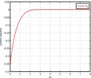
As shown in Fig.1, the curve represents the simulation result of state variablex0of subsystem
(6). It is obvious that the statex0can converge to zero at fixed time with the action ofu0, which is
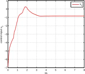
represented in Fig.2. Then, the states variablesx1,x2, andx3of the system (13) with respect to time
are reveled in Fig.3. The Fig.3 can illustrate that the states variablesx1,x2, andx3stabilized to zero
in fixed-time with the action of controlleru1obviously. And the controlleru1with respect to time is
shown in Fig.4. Thus, based on Figs.1-4, we can know that the controllersu0andu1can guarantee the
states of system (1) stabilization within fixed time.
0 1 2 3 4 5 6 7 8 −0.05
0 0.05 0.1 0.15 0.2
state/m
t/s
x
0
Figure 1.System statex0with respect to time.
0 1 2 3 4 5 6 7 8 −0.4
−0.35 −0.3 −0.25 −0.2 −0.15 −0.1 −0.05 0 0.05
control input/m
t/s
u0
Figure 2.Controlleru0with respect to time.
5. Conclusion
0 1 2 3 4 5 6 7 8 −0.8
−0.6 −0.4 −0.2 0 0.2 0.4 0.6
states/m
t/s
x1 x2 x3
Figure 3.System statex1,x2, andx3with respect to time.
0 1 2 3 4 5 6 7 8 −7
−6 −5 −4 −3 −2 −1 0 1
control input u
1
t/s
u1
Figure 4.Controlleru1with respect to time.
Author Contributions: Liang Zhenying contributed to the conception of the study.
Guo Pengfei contributed significantly to analysis, manuscript preparation and wrote the manuscript; Wang Xi and Jin Zengke helped perform the analysis with constructive discussions
Funding:This work was supported by (1)Provincial Natural Science Fund Project(ZR2014FM017, ZR2017LF011), (2)Shandong University of Technology Ph.D Startup Foundation(Grant NO.418048).
Conflicts of Interest:The authors declare no conflict of interest.
Abbreviations
The following abbreviations are used in this manuscript:
MDPI Multidisciplinary Digital Publishing Institute DOAJ Directory of open access journals
TLA Three letter acronym LD linear dichroism
References
1. A. M. Bloch, M. Reyhanoglu, N. H. Mcclamroch, Control and stabilization of nonholonomic dynamic systems. IEEE Transactions on Automatic Control, 37 (11) (1992) 1746-1757.
2. S. S. Ge, Z. Wang, T. H. Lee, Adaptive stabilization of uncertain nonholonomic systems by state and output feedback. Automatic, 39 (8) (2003) 1451-1460.
3. G. A. Lafferriere, E. D. Sontag, Remarks on control lyapunov functions for discontinuous stabilizing feedback. IEEE Conference on Decision & Control (1993)
5. S. P. Bhat, D. S. Bernstein, Geometric homogeneity with applications to finite-time stability.Mathematics of Control Signals and Systems17 (2) (2005) 101-127.
6. M. Defoort, M. Djemai, Finite-time controller design for nonholonomic mobile robot using the heisenberg formIEEE International Conference on Control Applications(2010).
7. J. J. Xiong, G. B. Zhang, Global fast dynamic terminal sliding mode control for a quadrotor uav.Isa Transactions 66 (2016) 233. 14
8. H. Zhang, Q. Qu, G. Xiao, Y. Cui, Optimal guaranteed cost sliding mode control for constrained-input nonlinear systems with matched and unmatched disturbances. IEEE Transactions on Neural Networks & Learning Systems29 (6) (2018) 1-15.
9. J. E. Solanes, L. Gracia, P. Mu ˜noz-Benavent, J. V. Miro, V. Girbs, J. Tornero, Human-robot cooperation for robust surface treatment using non-conventional sliding mode control. Isa Transactions(2018)
10. M. P. Aghababa, H. P. Aghababa, A novel finite-time sliding mode controller for synchronization of chaotic systems with input nonlinearity. Ara- bian Journal for Science & Engineering38 (11) (2013) 3221-3232. 11. Y. Hong, J. Wang, Z. Xi, Stabilization of uncertain chained form systems within finite settling time. IEEE
Transactions on Automatic Control50 (9) (2005) 1379-1384.
12. A. Polyakov, Nonlinear feedback design for fixed-time stabilization of linear control systems. IEEE Transactions on Automatic Control57 (8) (2012) 2106-2110.
13. Z. Zuo, T. Lin, Distributed robust finite-time nonlinear consensus protocols for multi-agent systems. International Journal of Systems Science47 (6) (2016) 1366-1375.
14. Z. Zuo, T. Lin, A new class of finite-time nonlinear consensus protocols for multi-agent systems. International Journal of Control87 (2) (2014) 363-370.
15. S. E. Parsegov, A. E. Polyakov, P. S. Shcherbakov, Fixed-time consensus algorithm for multi-agent systems with integrator dynamics. IFAC Pro- ceedings Volumes46 (27) (2013) 110-115.
16. Z. Zuo, Non-singular fixed-time terminal sliding mode control of nonlinear systems. Control Theory & Applications Iet9 (4) (2014) 545-552.
17. A. Levant, Robust exact differentiation via sliding mode technique. Automatica34 (3) (1998) 379-384. 18. E. Cruz-Zavala, J. A. Moreno, L. M. Fridman, Uniform robust exact differentiator. IEEE Transactions on
Automatic Control56 (11) (2011) 2727-2733.
19. W. Huang, Y. Yang, C. Hua, Fixed-time tracking control approach design for nonholonomic mobile robot. Control Conference2016, pp. 3423-3428.
20. M. Zheng, L. Li, H. Peng, J. Xiao, Y. Yang, Y. Zhang, Fixed-time synchronization of memristive fuzzy bam cellular neural networks with time-varying delays based on feedback controllers.IEEE AccessPP (99) 12085-12102.