University of Windsor University of Windsor
Scholarship at UWindsor
Scholarship at UWindsor
Electronic Theses and Dissertations Theses, Dissertations, and Major Papers
2018
An Adaptive Clustering Algorithm for Gene Expression
An Adaptive Clustering Algorithm for Gene Expression
Time-Series Data Analysis
Series Data Analysis
Naveen Mangalakumar
University of Windsor
Follow this and additional works at: https://scholar.uwindsor.ca/etd
Recommended Citation Recommended Citation
Mangalakumar, Naveen, "An Adaptive Clustering Algorithm for Gene Expression Time-Series Data Analysis" (2018). Electronic Theses and Dissertations. 7380.
https://scholar.uwindsor.ca/etd/7380
An Adaptive Clustering Algorithm for Gene
Expression Time-Series Data Analysis
By
Naveen Mangalakumar
A Thesis
Submitted to the Faculty of Graduate Studies through the School of Computer Science in Partial Fulfillment of the Requirements for
the Degree of Master of Science at the University of Windsor
Windsor, Ontario, Canada
2017
c
An Adaptive Clustering Algorithm for Gene Expression Time-Series Data Analysis
by
Naveen Mangalakumar
APPROVED BY:
A. Swan
Department of Biological Sciences
M. Kargar
School of Computer Science
L. Rueda, Advisor School of Computer Science
A. Ngom, Co-Advisor School of Computer Science
DECLARATION OF ORIGINALITY
I hereby certify that I am the sole author of this thesis and that no part of this thesis
has been published or submitted for publication.
I certify that, to the best of my knowledge, my thesis does not infringe upon anyones
copyright nor violate any proprietary rights and that any ideas, techniques, quotations, or any
other material from the work of other people included in my thesis, published or otherwise,
are fully acknowledged in accordance with the standard referencing practices. Furthermore,
to the extent that I have included copyrighted material that surpasses the bounds of fair
dealing within the meaning of the Canada Copyright Act, I certify that I have obtained a
written permission from the copyright owner(s) to include such material(s) in my thesis and
have included copies of such copyright clearances to my appendix.
I declare that this is a true copy of my thesis, including any final revisions, as approved
by my thesis committee and the Graduate Studies office, and that this thesis has not been
ABSTRACT
Studying gene expression through various time intervals of breast cancer survival may
provide insights into the recovery of the patients. In this work, we propose a hierarchical
clustering method used to separate dissimilar groups of genes in time-series data, which
have the furthest distances from the rest of the genes throughout different time intervals.
The isolated outliers(genes that trend differently from other genes) can serve as potential
biomarkers of breast cancer survivability. We partition the time axis (time points) into bins
of length six months starting from 1-6 up to 337-342 month intervals and, for each gene, we
average its expression level over all patients who appear in a survival bin. Gene expressions
throughout those time points are cubic spline interpolated to create a trending profile for
each gene. First, we universally align the gene expression profiles to minimize the total area
between them. Then, we cluster them using a sliding window approach and hierarchical
clustering based on minimum vertical distances. To the best of our knowledge, this work is
the first time-series model that is built on the survival time of patients after the treatment.
With this approach, we identified 46 genes (including 24 oncogenes and 18 tumor suppressor
DEDICATION
ACKNOWLEDGEMENTS
I would like to express my most profound gratitude to my supervisor Dr.Luis Rueda and
co-supervisor Dr.Alioune Ngom for their continuous support and guidance. The
brainstorm-ing sessions we had throughout this course taught me how to approach a problem like a
researcher. Thank you so much for being patient and giving me the liberty to explore my
new ideas; without your help, I would have never been able to complete this thesis.
Special thanks to my external reader Dr.Andrew Swan and my internal reader Dr.Mehdi
Kargar for their inputs and valuable suggestions to this work.
I'm grateful to my mentors Abedalrhman Alkhateeb and Huy Quang Pham for their
guidance and motivation, which gave a good start for my research. I enjoyed working with
you guys; it was a high learning curve.
Finally, I would like to thank my friends Uday, Venkat, Gouthaam, and Kamal for
TABLE OF CONTENTS
DECLARATION OF ORIGINALITY III
ABSTRACT IV
DEDICATION V
ACKNOWLEDGEMENTS VI
LIST OF FIGURES IX
LIST OF TABLES XII
1 Introduction 1
1.1 Breast Cancer . . . 1
1.2 Problem Statement . . . 4
1.3 Motivation . . . 5
1.4 Conclusion . . . 6
2 Literature Review 7 2.1 Contribution . . . 9
3 Materials and Methods 11 3.1 Dataset . . . 11
3.2 Preprocessing : Creating Time-Series . . . 12
3.3 Time-Series Interpolation Methods . . . 13
3.4 Clustering . . . 15
3.5 Our Baseline Method . . . 16
3.5.1 Natural Cubic Spline Interpolation . . . 16
3.5.2 Universal Alignment of Gene Profiles . . . 17
3.5.3 Distance Function . . . 17
3.5.4 Clustering Algorithm . . . 17
3.5.5 Profile Alignment and Agglomerative Clustering Index . . . 18
3.6 Workflow of Our Baseline Method . . . 19
3.7 Adaptive Clustering Algorithm . . . 19
3.8 Workflow of Proposed Algorithm . . . 20
3.8.1 Window Size for the First Iteration . . . 21
3.8.2 Step Size = 2 . . . 22
4 Computational Experiments and Results 26
4.1 Identifying the Window size for the first Iteration . . . 26
4.2 Results of the Baseline Method . . . 27
4.3 Adaptive Clustering Algorithm . . . 28
4.4 Comparison with other Approaches . . . 31
4.4.1 BiClustering using BiGGEsTS . . . 31
4.5 Adaptive Clustering Algorithm with k-means . . . 34
4.6 BiClustering in Scikitlearn . . . 34
4.7 Biological Insight . . . 35
4.7.1 Baseline Method . . . 35
4.7.2 Adaptive Clustering Algorithm . . . 36
4.8 Summary of results . . . 38
5 Conclusion and Future Work 40 5.1 Contributions . . . 41
5.2 Future Work . . . 41
REFERENCES 42
APPENDIX A Clustering results - Adaptive Clustering Algorithm 50
APPENDIX B Oncogenes 54
APPENDIX C Tumour Suppressor Genes 68
LIST OF FIGURES
1 Understanding cancer. . . 1
2 Central dogma of molecular biology. . . 3
3 Local and global outliers. . . 5
4 Creating time-series dataset. . . 12
5 Differrent interpolation methods.. . . 14
6 Clustering with complete linkage. . . 15
7 Workflow of our baseline method. . . 19
8 Slicing the time series based on Window size and Step size. . . 20
9 Workflow of the proposed algorithm. . . 21
10 Window size for the first iteration. . . 22
11 Change in gene trend. . . 23
12 Step size from iteration 2 onwards. . . 24
13 ACTS pseudocode. . . 25
14 Window size for the first iteration. . . 27
15 bicluster 672447 - the green line shows the trend of SCGBA2.. . . 32
16 bicluster 671866 - the green and yellow lines show the trend of SCGB1D2 and SCGB2A1 respectively. . . 32
17 bicluster 671471, cyan line shows the trend of ANKRDD30A. . . 33
18 Clustering results of ACTS for genes SCGBA2, SCGB1D2, SCGB2A1, ANKRD30A. 33 19 Expression of oncogenes and tumour suppressor genes. . . 37
20 Clustering results Window 1. . . 50
22 Clustering results Window 3. . . 51
23 Clustering results Window 6. . . 52
24 Clustering Results Window 7. . . 52
25 Clustering results Window 14. . . 52
26 Clustering results Window 15. . . 53
27 Clustering results Window 22. . . 53
28 Gene trend of SCGB2A2. . . 54
29 Gene trend of ANKRD30A. . . 55
30 Gene trend of SCGB1D2. . . 55
31 Gene trend of SCGB2A1. . . 56
32 Gene trend of PIP. . . 56
33 Gene trend of TFF3. . . 57
34 Gene trend of KRT81. . . 57
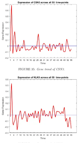
35 Gene trend of CSN3. . . 58
36 Gene trend of KLK5. . . 58
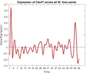
37 Gene trend of c4orf7. . . 59
38 Gene trend of BEX1. . . 59
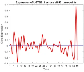
39 Gene trend of UGT2B11.. . . 60
40 Gene trend of UGT2B27.. . . 60
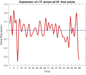
41 Gene trend of LTF. . . 61
42 Gene trend of UG2B28. . . 61
43 Gene trend of PROM1. . . 62
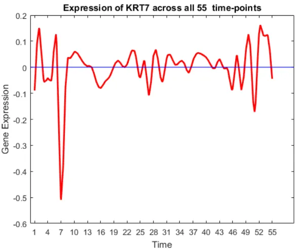
44 Gene trend of KRT7. . . 62
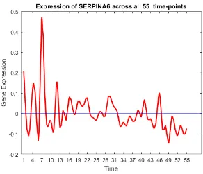
45 Gene trend of SERPINA6. . . 63
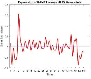
47 Gene trend of RAMP1. . . 65
48 Gene trend of CST1. . . 65
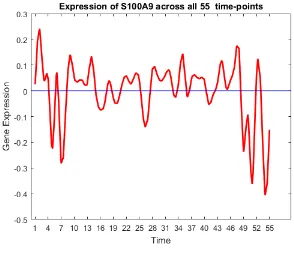
49 Gene trend of S100A9. . . 66
50 Gene trend of S100A8. . . 66
51 Gene trend of FLJ23152. . . 67
52 Gene trend of TAT. . . 68
53 Gene trend of BAMBI. . . 69
54 Gene trend of VTCN1. . . 69
55 Gene trend of HLA-DRB1. . . 70
56 Gene trend of PXDNL. . . 70
57 Gene trend of DIO1. . . 71
58 Gene trend of HSPB8. . . 71
59 Gene trend of CYP4X1. . . 72
60 Gene trend of HMGCS2. . . 72
61 Gene trend of CYP4Z1. . . 73
62 Gene trend of TFAP2B. . . 73
63 Gene trend of TFF1. . . 74
64 Gene trend of GRIA2. . . 74
65 Gene trend of EEF1A2. . . 75
66 Gene trend of BMPR1B. . . 75
67 Gene trend of MYBPC1. . . 76
68 Gene trend of SLC27A2. . . 76
LIST OF TABLES
1 Layout of our time series dataset. . . 13
2 Results of baseline method. . . 28
3 Outliers in each interval. . . 29
4 Genes filtered out as outliers in each interval. . . 30
CHAPTER 1
Introduction
1.1
Breast Cancer
What is Cancer?
Cells are basic functional and structural units of a living organism. A human body has
trillions of cells that act as building blocks to form tissues and organs in the human body.
Cells grow and multiply as and when the body demands. They also have the ability and
mechanisms to repair themselves when damaged or die when they are unable to. When a cell
dies, a new cell replaces it, and this process happens in an orderly and controlled fashion.
FIGURE 1: Understanding cancer.
Cancer is a disease that is characterized by uncontrolled cell growth in an organ. Figure
change in the structure of DNA (Deoxyribonucleic acid) in a cell that creates a mutation.
These mutated cells divide out of control and crowd out the healthy cells in the body. These
mutated cells also grow and form a tumor which can be cancerous or benign. A cancerous
tumor is malignant as it can grow and spread to other parts of the body, whereas a benign
tumor can grow but will not spread.
What is breast cancer?
Cancer can occur anywhere in the body as cells are everywhere in the body. Breast cancer
is the most common female cancer in the western world and one of the leading causes of
death by cancer among women. It stands second among the most prominent causes of death
amongst the middle-aged women in the world and most common in women over 50 years
of age [2, 18, 35, 69]. Breast cancer refers to a malignant tumor that has originated from
the cells of the breast. Recent studies showed that there exists extensive diversity between
and within breast cancer patients, while each breast cancer shows unique characteristics.
The heterogeneity of cancer complicates diagnosis and treatment [5]. Every person's cancer
develops uniquely and their responses to therapies are not the same. Breast cancer is caused
due to a genetic irregularity which occurs due to damaged DNA in a cell. Genomes are pieces
of DNA (deoxyribonucleic acid) inside a cell that instructs the cell what to do and when to
grow and divide. Each cell has about 25,000 genes in it [1]. Mutations in a small number of
genes, oncogenes or tumor suppressors, whose change deregulate many biological processes
leads to initiation and progression of breast cancer as well as resistance to treatment [31].
Figure 2 depicts the central dogma of molecular biology [4]. The red cross in the figure
shows the damaged DNA being used in transcription and translation processes. Gene
ex-pression is a process in which instructions in a DNA (i.e., genes) are converted into proteins
FIGURE 2: Central dogma of molecular biology.
changes in the environment. Transcription and translation are the most critical processes in
the conversion of a gene to protein. Transcription makes a mRNA (messenger RNA) molecule
which has instructions encoded in it for protein synthesis. Translation is the process of
de-coding the instructions on a mRNA to assemble a protein. Gene expression profiling is a
Biomarkers
A biomarker is defined as a measurable indicator of a biological process. There are five
distinct kinds of cancer biomarkers:
• Prognostic biomarkers: those that predict the development of cancer [30].
• Diagnostic biomarkers: those that predict the presence of disease or condition of in-terest or the subtype of cancer [47].
• Predictive biomarkers: those that predict the survivability of patient treated with the specific drug [22].
• Progression biomarkers: those that predict whether the cancer is spreading or not.
• Recurrence biomarkers: those that predict whether cancer will recur after sometime [70].
In this thesis, we define survivability as the period a treated patient lives after the first
diagnosis of the disease. Thus, we focus on finding predictive biomarkers that can help us
predict survivability of breast cancer patients from gene expression time-series data.
1.2
Problem Statement
Given a breast cancer dataset of patients of different survival status (living/dead), overall
survival time, type of treatment and subtype, we aim to :
• Create a time-series dataset of patients using the overall survival in the dataset based on survival status.
• Determine the exact time point at which the outlier (gene) is under-expressed/over-expressed.
Figure 3 depicts global and local outliers. Let us consider the curves as gene expression
profiles. From the beginning, the curve in red colour clearly trends different from other
curves. So this is a global outlier. The curve in yellow colour follows a similar trend with
other curves upto a certain point (represented by dotted lines) and starts following a different
trend. This is called a local outlier.
FIGURE 3: Local and global outliers.
1.3
Motivation
The discovery of biomarkers can be a crucial step in predicting survivability and handling of
expression values are different in various stages of progression of the disease. One of the
most powerful applications of gene expression analysis is to identify biomarkers that can be
used for disease risk assessment, early detection, prognosis and preventive measures [79]. In
the field of bioinformatics, in the recent years, researchers have spent lots of time and effort
in finding the biomarkers of different types of cancer at the genetic level. Genes tend to
under-express or over-express during progression and recurrence of any disease, especially
cancer. The problem of choosing those biomarker genes that provide insights about the
disease poses a challenging problem in high-dimensional data.
Previous work on detecting biomarkers at a gene level was focussed on grouping up of
similar gene expression profiles and eliminating the outlier genes as noise. In this thesis, we
propose a novel method to identify the genes that are dissimilar, as outlier genes, that can
serve as potential biomarkers of breast cancer survivability.
1.4
Conclusion
In this chapter, we discussed some important terminologies of breast cancer, the problem
statement and motivation for this thesis.
This thesis is organized as follows,
• In Chapter 2, we present the literature review.
• In Chapter 3, we introduce the materials and methods for this work.
• Chapter 4 contains details of computational experiments, results and discussion.
CHAPTER 2
Literature Review
Once a patient is diagnosed with breast cancer, one of the most challenging questions in
patient management are how to maximize the chances of survival with a chosen treatment.
Biomarkers identified using various methods discussed here are expected to provide more
accurate information to address this question. The following review helps us understand the
way biomarkers can be used to answer different clinical questions such as survival, disease
subtype and prognosis of a breast cancer patient. A relevant biomarker (gene in our case)
must be sensitive, specific, highly standardized and reproducible [79].
Yousef et al. [79] gave a review of various machine learning techniques such as clustering
and support vector machines (SVM), which are most commonly used for biomarker discovery.
They discussed various supervised, unsupervised learning and feature selection algorithms
in machine learning. They conclude that the best data mining approach to find biomarkers
would be to integrate different methods to arrive at an effective and efficient algorithm. They
also suggest incorporating biological knowledge in the algorithm to achieve more accurate
biological results.
Chen et al. [15] developed a network-constrained SVM algorithm for identifying cancer
biomarkers by integrating gene expression data and protein-protein interaction (PPI) data.
In this method, the clinical outcome of patients is predicted, and meaningful biomarkers
on gene-expression data and PPI network as input for predicting the outcome of new
sam-ples. Biomarkers were obtained by significance test based on permutation of sample labels.
These biomarkers had very high functional relevance to breast cancer and revealed potential
signaling pathways associated with breast cancer metastasis.
Swan et al. [67] used machine learning on proteomics data for biomarker identification.
In that paper, they used a process called peak picking (as part of preprocessing), which
checks the mass spectrometry data for peaks with significantly high signal intensities. These
peaks are considered as potential biomarkers (proteins), followed by using machine learning
techniques to identify the most suitable biomarkers. However, the drawback here is, the
results need further analysis. Also, additional preprocessing steps such as normalization,
peak alignment, and noise reduction techniques are essential to improve accuracy and avoid
errors.
Weiler et al. [43] developed a maximum difference subset algorithm that combines
classi-fication algorithm, statistics, and machine learning techniques. They described the goals of
data analysis in three steps (a) class discovery, (b) class prediction and (c) detecting
dysreg-ulated genes that trend different from other genes in the same subtype. The authors explore
the possibility that a clustering algorithm can be used in conjunction with a classical
statis-tical analysis in such way that considers classification accuracy for finding the dysregulated
genes. With this technique, they found five genes that were relevant to leukemia.
Miloli et al. [47] developed an algorithm that uses a new method called CM1 score
to identify biomarkers for subtype classification. CM1 score is a method to evaluate the
difference in expression levels of two samples in two classes. With this technique, they
identified 30 biomarkers for predicting breast cancer subtypes.
Alkhateeb et al. [9] proposed a time-series method to interpolate transcript expression
values over cancer stages to isolate outliers as biomarkers for prostate cancer. They used
from the other genes that follow a similar trend. They suggest that a combination of proper
clustering algorithm, suitable distance function and validity index is the best approach to
solve the problem of outlier detection.
Another approach is biclustering which reveals groups of genes that show similar activity
patterns under a specific subset of experimental conditions [45]. They deployed an open
source tool designed by Madeira et al., BiGGEsTS to analyze our gene-expression
time-series data [27]. However, there are some drawbacks with the tool:
• It only selects a subset of genes under specific conditions and subset of conditions under specific genes based on discretized matrix
• BiGGEsTS could not group all the genes with similar trend in one bicluster because of its Discretized matrix technique
• BiGGEsTS could not capture the change in gene-expression trend accurately.
• Single gene can occur in many biclusters.
BiClustering in Scikitlearn is another algorithm and involves a process in which rows and
columns of a dataset are clustered simultaneously. The clusters of rows and columns are
known as biclusters. Each determines a submatrix of the original data matrix with some
desired properties [52].
The literature suggests that most of the researchers have used clustering algorithms on
the data to pick relevant outliers as biomarkers for a disease.
2.1
Contribution
In this thesis, we propose an adaptive clustering algorithm to detect biomarkers of breast
• Creating a patient time-series data give gene expression data based on overall survival of breast cancer patients.
• Multiple alignment of gene expression profiles based on their trend across time-series.
CHAPTER 3
Materials and Methods
Machine Learning
Machine learning is a branch of artificial intelligence that provides various methods and
algorithms that are trained on inputs, and a model is extracted from them [71]. Subsequently,
that model is tested on a different set of inputs, and then the algorithm performance is
measured [71]. Clustering is an unsupervised technique in machine learning [71].
3.1
Dataset
The dataset used for this thesis is the Molecular Taxonomy of Breast Cancer
Interna-tional Consortium (METABRIC) dataset [19], which is publicly available at cBioPortal [3].
METABRIC is a Canada-UK project that aims to classify breast tumors into further
sub-categories, based on molecular signatures that helps determine the best course of treatment
to improve patients survivability. This dataset contains clinical data (Patient ID, Survival
status, overall survival in months and type of treatment) for a total of 1,904 patients. Of
these, 480 patients were diagnosed/treated for breast cancer but died because of some other
reason; thus,we filtered them out as they will have no relevance to our problem of predicting
biomarkers of survivability. That gives us a total of 1,424 patients; from which we consider
of survivability. The dataset has also expression data (24,368 genes determined through
microarray) for all the patients in the clinical dataset.
3.2
Preprocessing : Creating Time-Series
In preprocessing, first, the two datasets (clinical dataset and the gene expression dataset)
were merged with the KEY = PATIENT-ID, and next, we create a time-series. A time-series
is a sequence of measures at specific time points. Gene expression of cancer patients can be
measured at different time points. Also, time points can be interpolated to approximate the
growth of disease over time and isolate outliers.
Figure 4 depicts the process by which our time series data were created. The dataset
has patients overall survival (the day patients were diagnosed with breast cancer to the day
the dataset was created) in months. In this work, we assume the survival of each patient
as time-series. The shortest time of patient who survived is one month and the longest
being 342. To create the time-series data, we partition the time axis into survival bins of
length 6 months. We chose an interval of 6 months since the average time for progression of
cancer is 6 months. Also, for a cancer patient who is undergoing treatment, it takes at least
3-6 months to respond to it. For the dataset we have, time series starts from 1-6 months,
7-12 months and go on until 337-342, giving us 55 time points. Next, we average the gene
expression levels over all the patients appearing in a survival bin. Table 1 depicts the layout
of our time series dataset with 24,368 rows × 55 columns. Time-point 1
(1 - 6 months)
Time-point 2
(7 - 12 months) ...
Time-point 55
(337 - 342 months)
Gene 1
Average of (Gene 1 in
1-6 Months bin)
Average of (Gene 1 in
7-12 Months bin)
...
Average of (Gene 1 in
337-342 Months bin)
Gene 2 . . ... .
Gene 3 . . ... .
Gene 4 . . ... .
Gene 24368
Average of (Gene
24368 in 1-6 Months
bin)
Average of (Gene
24368 in 7-12 Months
bin)
...
Average of (Gene
24368 in 337-342
Months bin)
TABLE 1: Layout of our time series dataset.
3.3
Time-Series Interpolation Methods
Interpolation is defined as the method of constructing new data points within a range of
already known data points [74]. There are four different methods to interpolate time-series
data:
assigning that to unknown data value [74].
• Linear Interpolation(Figure 5b) - is to use linear polynomials to construct new data points within the range of a discrete set of known data points [74].
• Polynomial Interpolation (Figure 5c) - is the interpolation of a given data set by the polynomial of degreed >0 that passes through the points of the dataset [74].
• Spline Interpolation(Figure 5d) - Spline interpolation uses cubic polynomials in each of the intervals and chooses the polynomials such that they fit smoothly together [74].
In this work, we use spline interpolation, since it is more accurate and computationally
less expensive.
3.4
Clustering
A cluster is defined as a collection of objects that are similar to each other and are dissimilar
to the objects belonging to other clusters.
In this thesis, we use hierarchical agglomerative clustering which is a distance-based and
a bottom-up approach. Before performing clustering, it is important to determine the
dis-tance matrix, which shows the disdis-tance between each pair of points using a disdis-tance function.
This matrix is updated each time two points are clustered together. There are different ways
by which the distance or the proximity between clusters is measured. This process is called
linkage. In this thesis, we are using complete linkage (Figure 6) or furthest neighbors, which
computes the distance between the furthest pair of points for each pair of clusters and merges
the pair of clusters that have the minimum furthest distance among all such distances
be-tween the pair of clusters under consideration [56].
3.5
Our Baseline Method
We propose an approach to identify biomarkers in breast cancer progression from outliers of
time-series clusters. We study the progression of breast cancer by identifying the biomarkers
in gene-expression profiles throughout various time-points created based on patient survival.
We propose an algorithm which is a combination of a cubic spline interpolation, universal
profile alignment, a distance function, a clustering algorithm to detect outliers, and a cluster
validity index (PAAC) to determine the best number of clusters for the dataset. Each of
these functions is discussed in detail below.
3.5.1
Natural Cubic Spline Interpolation
Gene expressions throughout the time points are natural cubic spline interpolated to create
a trending profile for each gene in the given dataset [9, 62, 65, 66]. For profile x(t), where tis
a vector that represents time points [t1, t2, ., tn], x(t) is interpolated continuously as follows:
x(t) =
x1(t), if t1 ≤t ≤t2 xj(t), if tj < t≤tj+1 xn−1(t), if tn−1 < t≤tn
where xj(t) =xj3(t−tj)3+xj2(t−tj)2 +xj1(t−tj)1+xj0(t−tj)0
xj(t) interpolates x(t) in the interval [tj, t(j + 1)], with spline coefficients xjk ∈ R, for 1 ≤j ≤n−1 and 0 ≤ k ≤ 3. The interpolated x(t) spline has a natural condition, which means that the first and second derivatives of the spline at each interval x(t) are equal to
3.5.2
Universal Alignment of Gene Profiles
Given a datasetX ={x1(t), x2(t), .. xm(t)}where mis the number of profiles, cubic splines
profiles were universally aligned by shifting the interpolated gene profiles vertically in such
a way that the squared error between any two of those profiles is minimal [9, 56, 62, 65, 66].
Pairwise alignment for all possible pairs of profiles is done by aligning all profiles to a profile
z(t) = 0 (universal alignment).
3.5.3
Distance Function
The distance between the two profiles x(t) and y(t) is the area d(x,y) between those two
profiles after universal alignment as per the equation below:
d(x, y) =
Z tn
0
[x(t)−y(t)].dt
The distance between two profiles is the area between the two profiles after shifting the
profiles vertically in such a way to obtain the minimum possible area between them. All the
profiles are aligned to the universal profilez(t) (universal alignment) in such a way that the
area between z(t) and the profile is minimum [9, 56, 62, 65, 66].
3.5.4
Clustering Algorithm
The main objective of using clustering here is to filter out the profiles that trend differently
from other profiles [9, 62, 65, 66]. In this work, we have chosen singleton clusters as outliers.
We also choose clusters with a very small number of profiles that follow the same trend with
profiles within the cluster and dissimilar from other profiles in a different cluster. Hierarchical
agglomerative clustering is a bottom-up approach. Initially, each profile in the dataset is
an individual cluster (each profile is a cluster), and then the clusters are merged based on
criteria (computing the distance between the furthest pair of points for each pair of clusters
and combines the pair of clusters that has the minimum furthest distance among all such
distances). The merging process continues until the desired number of clusters is reached.
This approach places the profiles with similar trends into one cluster and filters out profiles
that are less similar to other profiles as one or more different clusters.
3.5.5
Profile Alignment and Agglomerative Clustering Index
Profile alignment and agglomerative clustering Index (PAAC) [9, 62, 65, 66] is the validity
index that has been used to determine the desired number of clusters for the dataset. PAAC
is a modified version of the I-index [29]. Rueda et al. modified the I-Index formula to reduce
the impact the I-index value faces when many clusters are used in it as follows:
I(k) = (1 k)
q×(B
W ×D)
p,
where:
D= (maxi,j=1)kd(µi, µj),
B =
k
P
i<c
d(µi, µc),
W = k P i=1 n P j=1
µijd(xj, µi),
k is the number of clusters,q is the coefficient of normalizing the number of clusters,pis
the coefficient of the degree of the index,µij = 1 if genejbelongs to theith cluster; otherwise
µij = 0, µi is the center of ith cluster, n is the number of genes, and d(. , .) is the distance
3.6
Workflow of Our Baseline Method
In our baseline method, the entire time-series dataset (time point 1 to time point 55) is
universally aligned towards the universal profile z(t). Then, we use hierarchical clustering
to detect the gene profiles that trend differently from others. Finally, we use cubic spline
interpolation to identify singleton clusters that trend differently from other genes as outliers.
Figure 7 depicts the workflow of our baseline method.
FIGURE 7: Workflow of our baseline method.
3.7
Adaptive Clustering Algorithm
We propose an iterative adaptive clustering algorithm (ACTS) wherein we slice the time-axis
into distinct intervals based on three parameters, window size, outlier threshold and step size
(Figure 8). To detect the local and global outliers, it is essential to slice the time-series data
and perform the clustering algorithm on each interval separately and identify the outliers
based on the partial clustering results. Partially clustering the dataset makes our algorithm
to adapt to the structure of data in a specific interval and identifies the genes that are more
FIGURE 8: Slicing the time series based on Window size and Step size.
3.8
Workflow of Proposed Algorithm
Figure 9 depicts the work flow of the proposed algorithm. The proposed algorithm uses an
iterative approach to detect outliers as biomarkers. We first slice the time-series dataset
based on two parameters, Window size and Step size. Window size is chosen in a way
that covers the interval that has the largest variation among genes. Step size here is a
fixed parameter, which is equal to two. Outlier threshold is an arbitrary parameter used
to limit the number of outliers in each interval. Then, we use hierarchical clustering and
spline interpolation methods to detect outliers on each sliced interval based on an Outlier
FIGURE 9: Workflow of the proposed algorithm.
3.8.1
Window Size for the First Iteration
Window size for the first iteration/interval is decided based on visualizing the data. This
parameter is dynamic and highly dependent on the structure of the dataset. We choose
the window size in such a way that the interval has considerable gene expression variability
among the genes and, many visible peaks which could be potential outliers. A disease like
cancer during the progression has several genes that are over-expressed in the initial stage
of the disease. Thus, the main idea here is to pick many observations/genes that trend
iteration, the algorithm proceeds as follows:
• Extract data based on the window size from the time-series dataset.
• Perform multiple profile alignment and clustering to detect potential biomarkers within that interval. In Figure 10, based on visualization, we choose window size = 8 time
points for the first iteration in our time-series dataset.
FIGURE 10: Window size for the first iteration.
3.8.2
Step Size = 2
Step size here is a fixed parameter and is used from the second iteration onwards until the
last time-point in the dataset. Genes that are outliers trend differently from others. We
investigated all possible trends a gene could follow, to be captured as an outlier. In Figure
to determine if it is an outlier in an interval. From the second iteration onwards, the step
size is used to include new time-points from the dataset for the next consecutive iterations
until the last time-point is reached.
FIGURE 11: Change in gene trend.
After the first iteration, we proceed with the algorithm based on Step size = 2. Figure
12 depicts how step size is used in our time-series dataset. From the second iteration until
• Adds two points after each iteration until the last time-point in the dataset.
• Performs multiple profile alignment and clustering on each interval until the end.
FIGURE 12: Step size from iteration 2 onwards.
3.8.3
Outlier Threshold
Outlier threshold is an arbitrary parameter used to determine and limit the number of genes
in a cluster that can be filtered out as outliers. Alkhateeb et al. [9] used a threshold of one
gene in a cluster (singleton clusters). In our case, it is difficult to determine the local outliers
with a threshold of one gene in a cluster. With specific time intervals, it is not easy to filter
out singleton clusters as there could be many genes following a similar trend. Thus, we set
dissimilarity among the clustered data. Figure 13 contains the pseudo code for the proposed
algorithm.
1: Input: Time-Series Dataset,Window size, Step size, Outlier Threshold, k range 2: Output: Outliers in each interval
3:
4: input1 = Time-series Dataset (1:Window size) 5: clustering and PAAC(input1)
6:
7: repeat
8: input2 = new dataset;
9: clustering and PAAC(input2) 10: until last time point is reached 11:
12: function clustering and PAAC(input) 13: for each gene in input do
14: uni-align = Align each gene towards universal profile Z(t) 15: end for
16: for each value ink range do
17: perform Hierarchical Agglomerative Clustering of uni-align 18: perform PAAC to determine the best kvalue
19: end for
20: Choose k value for max(PAAC)
21: plot cubic spline Interpolation for best k value clustering result 22: if Cluster size ≤ Outlier Thresholdthen
23: filter genes in cluster as outliers 24: else
25: new dataset = Add time-points based on Step size for next iteration. 26: end if
27: end function
CHAPTER 4
Computational Experiments and
Results
4.1
Identifying the Window size for the first Iteration
For determining the window size for Iteration 1 we:
• Perform multiple alignment on the time-series dataset, and
• Visualize the dataset after multiple-alignment.
Figure 14 shows two plots. The graph on top depicts the gene-expressions data plotted
before alignment. The graph at the bottom (titled Universal Alignment towards thet−axis) contains gene-expressions aligned towards the Z(t) = 0 profile.
As discussed in Chapter 3, the main idea is to select a window size such that many
outliers are filtered out in the very first iteration. In Figure 14, Universal Alignment, it
is noticeable that some genes are over and under-expressed at the same time in the first 8
time-points (green peaks in between red dotted lines, above and below the zero axis).
This suggests that in initial stages, the over-expressed genes could characterize the
pro-gression of breast cancer. Also, genes that are filtered out in the first few iterations could
FIGURE 14: Window size for the first iteration.
suppressor genes) that could slow down the rate at which cancer progresses. From Figure 14,
we infer that up-regulation of genes/peaks towards the end suggests high activity of tumor
suppressor genes which helped the patients survive for a long time.
4.2
Results of the Baseline Method
We identified 24 genes, which could potentially serve as biomarkers of breast cancer
surviv-ability. These could serve as global outliers as per our problem statement, considering the
whole time-series dataset. With parameters q = 0.7,p = 2,k = 46 clusters, we obtained 24
S.No Gene Related to BC?
1 HIST1H4C X
2 ATP5EP2 X
3 PSAP X
4 CD81 X
5 RPS5 X
6 EEF1A1 X
7 PYY2 X
8 HES7 X
9 ZNF678 X
10 ATP5B X
11 RPL11 X
12 RPS20 X
13 SNRPD2 X
TABLE 2: Results of baseline method. (BC - Breast cancer)
S.No Gene Related to BC?
14 RPL32 X
15 HSP90B1 X
16 TOMM7 X
17 UBA52 X
18 BGN X
19 RPS15 X
20 RPL12 X
21 TIMP1 X
22 RPS16 X
23 FTL X
24 RPL10 X
4.3
Adaptive Clustering Algorithm
After running the ACTS, we found 53 genes as potential biomarkers of breast cancer
sur-vivability. The window size for Interval-1 is set to 8, step size is set to 2 from Interval-2
Window TP Genes Outliers
1 1...8 24368 4
2 1...10 24364 19
3 1...12 24345 9
4 1...14 24336
-5 1...16 24336
-6 1...18 24336 5
7 1...20 24331 5
8 1...22 24326
-9 1...24 24326
-10 1...26 24326
-11 1...28 24326
-12 1...30 24326
-13 1...32 24326
-14 1...34 24326 6
TABLE 3: Outliers in each interval. (TP-Time-points)
Window TP Genes Outliers
15 1...36 24320 4
16 1...38 24316
-17 1...40 24316
-18 1...42 24316
-19 1...44 24316
-20 1...46 24316
-21 1...48 24316
-22 1...50 24316 1
23 1...52 24315
-24 1...54 24315
-S.No TP Gene Rel. to BC?
1
1..8
SCGB2A2 X
2 ANKRD30A X
3 SCGB1D2 X
4 SCGB2A1 X
5
1..10
PIP X
6 TFF3 X
7 KRT81 X
8 CSN3 X
9 KLK5 X
10 C4orf7 X
11 TAT X
12 BEX1 X
13 UGT2B11 X
14 UGT2B7 X
15 LTF X
16 UGT2B28 X
17 LOC338579 X
18 PROM1 X
19 BAMBI X
20 VTCN1 X
21 KRT7 X
22 DQ893812 X
23 HLA-DRB1 X
24
1..12
DB005376 X
25 SERPINA6 X
26 PXDNL X
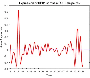
27 CPB1 X
TABLE 4: Genes filtered out as outliers in each interval.
S.No TP Gene Rel. to BC?
28 1..12 DIO1 X
29 HSPB8 X
30 RAMP1 X
31 CST1 X
32 FLJ23152 X
33
1..18
CYP4X1 X
34 HMGCS2 X
35 CYP4Z1 X
36 TFAP2B X
37 PPP1R1B X
38
1..20
TFF1 X
39 GRIA2 X
40 EEF1A2 X
41 BMPR1B X
42 CLIC6 X
43
1..34
TCN1 X
44 MYBPC1 X
45 CNTNAP2 X
46 S100A9 X
47 S100A8 X
48 S100P X
49
1..36
SLC27A2 X
50 PHGR1 X
51 SYT13 X
52 SERPINA5 X
53 1..50 TUBA3D X
4.4
Comparison with other Approaches
4.4.1
BiClustering using BiGGEsTS
We compared ACTS with the biclustering method proposed by Madeira et al. Unlike
cluster-ing, biclustering is a process in which rows and columns of a matrix are clustered
simultane-ously. BiGGEsTS created a total of 679,107 biclusters for our time-series dataset. BiGGesTS
selects specific intervals where a group of genes tends to over-express and clusters them
to-gether. The time intervals are chosen from anywhere in the dataset (beginning, middle or
end) without changing the order of time-series. Moreover, ACTS always clusters genes from
the beginning (time-point 1) and continues until the end based on step size. Thus, genes that
have the similar trend from the beginning are clustered together in ACTS, and genes that
have similar expression trend in a specific time interval are clustered together in BiGGEsTS.
From the results, we could see that ACTS has better performance than BiGGEsTS. Let
us consider the following example. Genes SCGB2A2, ANKRD30A, SCGB1D2, SCGB2A1,
follow similar trend from time-point 1 to time-point 8 in the given dataset. The results of
BiGGEsTS and ACTS are as follows:
• BiGGEsTS clustered the genes :
– SCGBA2 in bicluster - 672447 (Figure 15; the green line show the trend of
SCGBA2)
– SCGB1D2, SCGB2A1 in bicluster 671866 (Figure 16; the green and yellow lines
show the trend of SCGB1D2 and SCGB2A1 respectively)
FIGURE 15: bicluster 672447 - the green line shows the trend of SCGBA2.
FIGURE 17: bicluster 671471, cyan line shows the trend of ANKRDD30A.
Figure 18 depicts the clustering results of ACTS for the genes SCGBA2, SCGB1D2, SCGB2A1,
ANKRD30A. These genes were identified as outliers in the same cluster (highlighted in red)
after comparing it against the other 24368 genes. All clusters less than 5 genes(outlier
threshold) are plotted in red color.
BiGGEsTS failed to cluster them in the same bicluster as it could not capture the
simi-larity in gene trends across time. The discretization technique used in BiGGEsTS does not
take the gene-expression values but discretized values (D, N, U element in a data matrix
are replaced by a U if the difference between its expression value and the value in the same
gene and previous time point are higher than the threshold (=1), by a D if such difference
is lower than the symmetric of the threshold value, and N otherwise) while clustering rows
and columns. BiGGEsTS ignores the trend associated with each gene. However, ACTS
con-siders the trend created by gene-expression for clustering and hence gives better accuracy in
filtering out biomarkers.
4.5
Adaptive Clustering Algorithm with
k
-means
k-means clustering approach was used to compare the results of ACTS. k-means algorithm
despite being sensitive to outliers, failed to detect any outlier genes in the time-series dataset.
k-means clustering on each iteration kept clustering the genes to the nearest centroid ignoring
the minute change in gene trends across time. However, hierarchical clustering accurately
captured all the dissimilarities in genes taking even the slightest change in trend into account.
4.6
BiClustering in Scikitlearn
BiClustering algorithm in Scikitlearn [52] was also applied to the time-series dataset and
we observed that it is not suitable for data having any time component in it. Biclustering
changes the order of conditions/column/features when it clusters the dataset columnwise. In
our case, the columns are time intervals in months. The order of time must be preserved to
pick meaningful insights and making accurate predictions on the progression of any disease.
4.7
Biological Insight
Our baseline method detected 24 local outliers of which 14 genes were related to breast
can-cer survivability. ACTS detected 53 outliers, out of which 46 of them were related to breast
cancer. ACTS yields an accuracy of 86.7% in terms of clustering the potential
biomark-ers of breast cancer survivability. We identified 24 oncogenes and 18 tumour suppressor
genes. With the help of previous literature, we observe the biological significance of all genes
obtained as potential biomarkers of breast cancer survivability :
4.7.1
Baseline Method
• PSAP are related to breast cancer recurrence and potentiate resistance to breast cancer treatment [8].
• CD81 is a biomarker responsible for cancer proliferation [60].
• EEF1A1is an oncogene, a potential oncoprotein that is overexpressed in about two-thirds of breast tumours [68].
• HES7, SNRPD2, UBA52, RPL12 are genes that can affect the survival rate of breast cancer patients if highly expressed [6, 28, 29, 36, 55].
• RPL11, TIMP1, FTL and RPL32 are biomarkers of breast cancer development [12, 46, 82].
• HSP90B1 is an oncogene that is associated with breast cancer metastasis and de-creased survival [55].
• BGN is used for subtype-specific classification [81].
4.7.2
Adaptive Clustering Algorithm
• Oncogenes: SCGB2A2, ANKRD30A, SCGB1D2, SCGB2A1, TFF3, KRT81, CSN3, KLK5, C4orf7, BEX1, UGT2B11, UGT2B7, LTF, UGT2B28, PROM1, KRT7,
SER-PINA6, CPB1, RAMP1, CST1, FLJ23152, S100A9, S100A8 [11,13,14,17,20,24,25,33,
39, 42, 49, 51, 57, 58, 64, 72, 75, 78, 80, 81].
• Tumour Suppressor Genes: TAT, BAMBI, VTCN1, HLADRB1, PXDNL, DIO1, HSPB8, CYP4X1, HMGCS2, CYP4Z1, TFAP2B, TFF1, GRIA2, EEF1A2, BMPR1B,
MYBPC1, SLC27A2, SERPINA5 [7,10,16,21,26,32,37,38,48,53,54,59,61,63,73,76,77].
• SYT13 & TUBA3D are associated with ER specific cancer [23, 50].
• TCN1 There will be adverse effects on treatment if this gene is highly expressed [40].
• S100P Survival rate is decreased if this gene is highly expressed [44].
• PIP
– regulates proliferation of luminal-A type breast cancer cells in an estrogen-independent
manner [77].
– ER+ breast cancer, particularly those with very high level of ER expression, PIP
appears to play an important role in proliferation and invasion as well as acquired
resistance to tamoxifen [26].
– Biomarker in breast cancer micrometastasis [16] and outcome prediction in breast
carcinoma [51].
FIGURE 19: Expression of oncogenes and tumour suppressor genes.
Most of the oncogenes were over-expressed in the first and last few time-points. Some
tumour suppressor genes are underexpressed in the beginning, and most of them are
over-expressed at the end. The activity of tumour suppressor genes towards the end satisfies
the biological meaning of cancer, suggesting that the down-regulation of a set of genes may
be the underlying mechanism of cancer formation, while the up-regulation may characterize
and possibly control the state of evolution of individual cancers. Initially, the activity of
tumour suppressor genes was low, resulting in high activity of oncogenes, and hence the
pro-gression of the disease. Towards the end, more tumor suppressor genes are activated which
neutralizes the effect of oncogenes helping in patients increased survivability rate.
Since we know precisely at which time-point an oncogene is over-expressed, we can direct
or target treatments towards it to reduce/control their high activity which could improve
patients overall survivability. At the same time, any efforts to trigger or enhance the activity
of tumour suppressor genes could also contribute to increasing the rate of survivability during
4.8
Summary of results
We compared the results of our baseline method and ACTS with the other clustering methods
like biclustering with BiGGEsTS, biclustering in SckitLearn and k-means algorithm. Other
approaches failed to detect outliers as our method did. The results are summarized as follows:
• BiGGEsTS - created 679,107 biclusters for our time-series dataset. The tool does not detect the outliers and is not flexible enough to let us download the data created
in each bicluster. We had to visually check the bicluster to compare the outlier genes
from ACTS.
• Biclustering in ScikitLearn- is based on Python. This method is not recommended for data with time-series data as it does not preserve the order of time-series. The
algorithm alters the order of time-series while column-wise clustering.
• k-means Algorithm- could not filter outliers as it failed to detect the minute changes in gene trends across all the time points. The algorithm kept clustering genes on each
interval to the nearest centroid. Thus, there were no Outliers detected with k-means
clustering.
S.No Method Total Outliners Related to Breast Cancer Oncogenes Tumor Suppressor Genes Remarks
1 Baseline Method 24 14 12
-Clustered 14 of 24 global
biomarkers related to
breast cancer correctly
2 ACTS 53 46 24 18
Clustered 46 of 53
lo-cal biomarkers related to
breast cancer correctly
Parameters
• Order of time-series must always be preserved
• Determining theWindow size for the first iteration: This is an important parameter chosen at the beginning of the algorithm. Since it is an iterative algorithm, the initial
window size must be selected carefully after visualizing the dataset.
• Outlier threshold: This is a parameter that determines the accuracy of the clustering algorithm. We conducted a series of experiments to decide on the outlier threshold.
The outlier threshold must be chosen such that the biological meaning of the problem
is satisfied, and the results correspond to it.
CHAPTER 5
Conclusion and Future Work
In this thesis, we were given a clinical and gene-expression dataset of breast cancer patients.
We have developed an innovative approach to detect outliers (genes that trend differently
from the majority of other) as biomarkers of breast cancer survivability from this data using
a time-series model. These biomarkers can be used to predict and improve patient survival,
diagnosis, and therapy for breast cancer.
To solve this, we first created a time-series dataset using patients overall survival. We
grouped patients into survival bins based on their survival in months and averaged the gene
expression level of all the patients in each survival bin.
Then, we sliced the time series dataset with a sliding window approach to create
gene-expression data on specific intervals and used profile alignment and agglomerative clustering
in each interval to detect local outliers.
Finally, we found the biological relevance of genes closely related to breast cancer
sur-vivability suggesting them as potential biomarkers for wet-lab experiments. Our algorithm
detected 46 genes related to breast cancer survivability including 24 oncogenes and 18 tumor
5.1
Contributions
The main contributions of this thesis can be summarized as follows:
• We propose an adaptive clustering algorithm to detect biomarkers of breast cancer survivability using time-series data.
• We create a time-series with gene-expression data based on overall survival of breast cancer patients.
• Multiple alignment of gene expression profiles is based on their trend across time-series.
• ACTS (sliding window approach) is used to identify outliers (as biomarkers) in time-series data.
5.2
Future Work
• We have used the data from living patients in the dataset. ACTS can also be extended to the patients who died to pick biomarkers. We can compare the two results (living
and dead) and pull meaningful insights.
• Try this method on a different breast cancer dataset.
• Try this method on a different cancer dataset. e.g., prostate cancer data.
REFERENCES
[1] Breast cancer facts. http://www.cancerresearchuk.org/about-cancer/ what-is-cancer/genes-dna-and-cancer, 2017 (Last access : Sept 2017).
[2] Breast Cancer Facts. www.cancer.ca, 2017 (Last access : Sept 2017).
[3] cBioPortal. http://www.cbioportal.org/, 2017 (Last access : Sept 2017). Metabric dataset.
[4] Central dogma of biology.http://www.nationalbreastcancer.org/what-is-cancer, 2017 (Last access : Sept 2017).
[5] Image courtesy. http://www.nationalbreastcancer.org/what-is-cancer, 2017 (Last access : Sept 2017).
[6] J. Aaroe, T. Lindahl, V. Dumeaux, S. Saebo, D. Tobin, N. Hagen, P. Skaane, A. Lon-neborg, P. Sharma, and A.-L. Borresen-Dale. Gene expression profiling of peripheral blood cells for early detection of breast cancer. Breast Cancer Research, 12(1):R7, 2010.
[7] A. Al-Dwairi, F. A. Simmen, G. J. Fuchs, R. Hakkak, and S. Korourian. Dietary soy pro-tein induces hepatic lipogenic enzyme gene expression while suppressing hepatosteatosis in obese female zucker rats bearing dmba-initiated mammary tumors. Genes & Nutri-tion, 7(4):549, 2012.
[8] A. Ali, L. Creevey, Y. Hao, D. McCartan, P. OGaora, A. Hill, L. Young, and M. McIl-roy. Prosaposin activates the androgen receptor and potentiates resistance to endocrine treatment in breast cancer. Breast Cancer Research: BCR, 17(1), 2015.
[9] A. Alkhateeb, I. Rezaeian, S. Singireddy, and L. Rueda. Obtaining biomarkers in cancer progression from outliers of time-series clusters. In Bioinformatics and Biomedicine (BIBM), 2015 IEEE International Conference on, pages 889–896. IEEE, 2015.
[11] P. Bouchal, M. Dvoˇr´akov´a, T. Roumeliotis, Z. Bortl´ıˇcek, I. Ihnatov´a, I. Proch´azkov´a, J. T. Ho, J. Mary´aˇs, H. Imrichov´a, E. Budinsk´a, et al. Combined proteomics and tran-scriptomics identifies carboxypeptidase b1 and nuclear factor κB (NF-κB) associated proteins as putative biomarkers of metastasis in low grade breast cancer. Molecular & Cellular Proteomics, 14(7):1814–1830, 2015.
[12] T. R. Cawthorn, J. C. Moreno, M. Dharsee, D. Tran-Thanh, S. Ackloo, P. H. Zhu, G. Sardana, J. Chen, P. Kupchak, L. M. Jacks, et al. Proteomic analyses reveal high expression of decorin and endoplasmin (HSP90B1) are associated with breast cancer metastasis and decreased survival. PLOS one, 7(2):e30992, 2012.
[13] K. Chapman, J. Wagner, M. West, J. Kidd, and M. Prendes. Methods and composi-tions for the treatment and diagnosis of breast cancer, Aug. 21 2014. US Patent App. 14/238,726.
[14] C. Chen, Z. Li, Y. Yang, T. Xiang, W. Song, and S. Liu. Microarray expression profiling of dysregulated long non-coding rnas in triple-negative breast cancer. Cancer Biology & Therapy, 16(6):856–865, 2015.
[15] L. Chen, J. Xuan, R. B. Riggins, R. Clarke, and Y. Wang. Identifying cancer biomarkers by network-constrained support vector machines.BMC Systems Biology, 5(1):161, 2011.
[16] C. Choi, J. Choi, Y. Park, Y. Lee, S. Song, C. Sung, T. Song, M. Kim, T. Kim, J. Lee, et al. Identification of differentially expressed genes according to chemosensitivity in advanced ovarian serous adenocarcinomas: expression of GRIA2 predicts better survival. British Journal of Cancer, 107(1):91–99, 2012.
[17] Q.-Y. Chong, M.-L. You, V. Pandey, A. Banerjee, Y.-J. Chen, H.-M. Poh, M. Zhang, L. Ma, T. Zhu, S. Basappa, et al. Release of HER2 repression of trefoil factor 3 (TFF3) expression mediates trastuzumab resistance in HER2+/ER+ mammary carcinoma. On-cotarget, 8(43):74188, 2017.
[18] F. Coelho, A. de Padua Braga, R. Natowicz, and R. Rouzier. Semi-supervised model applied to the prediction of the response to preoperative chemotherapy for breast cancer. Soft Computing, 15(6):1137–1144, 2011.
[19] C. Curtis, S. P. Shah, S.-F. Chin, G. Turashvili, O. M. Rueda, M. J. Dunning, D. Speed, A. G. Lynch, S. Samarajiwa, Y. Yuan, et al. The genomic and transcriptomic archi-tecture of 2,000 breast tumours reveals novel subgroups. Nature, 486(7403):346–352, 2012.
[21] K. Dai, F. Qin, H. Zhang, X. Liu, C. Guo, M. Zhang, F. Gu, F. Li, and Y. Ma. Low expression of BMPRIB indicates poor prognosis of breast cancer and is insensitive to taxane-anthracycline chemotherapy. Oncotarget, 7(4):4770, 2016.
[22] P. Dao, K. Wang, C. Collins, M. Ester, A. Lapuk, and S. C. Sahinalp. Optimally discriminative subnetwork markers predict response to chemotherapy. Bioinformatics, 27(13):i205–i213, 2011.
[23] K. Datta, D. R. Hyduke, S. Suman, B.-H. Moon, M. D. Johnson, and A. J. Fornace. Exposure to ionizing radiation induced persistent gene expression changes in mouse mammary gland. Radiation Oncology, 7(1):205, 2012.
[24] J. J. de Ronde, E. H. Lips, L. Mulder, A. D. Vincent, J. Wesseling, M. Nieuwland, R. Kerkhoven, M.-J. T. V. Peeters, G. S. Sonke, S. Rodenhuis, et al. SERPINA6, BEX1, AGTR1, SLC26A3, and LAPTM4B are markers of resistance to neoadjuvant chemotherapy in HER2-negative breast cancer. Breast Cancer Research and Treatment, 137(1):213–223, 2013.
[25] M. Eisenblaetter, F. Flores-Borja, J. J. Lee, C. Wefers, H. Smith, R. Hueting, M. S. Cooper, P. J. Blower, D. Patel, M. Rodriguez-Justo, et al. Visualization of tumor-immune interaction-target-specific imaging of S100A8/A9 reveals pre-metastatic niche establishment. Theranostics, 7(9):2392, 2017.
[26] B. E. Gillesby and T. R. Zacharewski. PS2,TFF1 levels in human breast cancer tumor samples: correlation with clinical and histological prognostic markers. Breast Cancer Research and Treatment, 56(3):251–263, 1999.
[27] J. P. Gonccalves, S. C. Madeira, and A. L. Oliveira. Biggests: integrated environment for biclustering analysis of time series gene expression data. BMC Research Notes, 2(1):124, 2009.
[28] K. M. Goudarzi and M. S. LindstroM. Role of ribosomal protein mutations in tumor development. International Journal of Oncology, 48(4):1313–1324, 2016.
[29] K. A. Graham, X. Ge, A. de las Morenas, A. Tripathi, and C. L. Rosenberg. Gene expression profiles of estrogen receptor positive and estrogen receptor negative breast cancers are detectable in histologically normal epithelium. Clinical Cancer Research, pages clincanres–1369, 2010.
[30] M. E. Hahn and M. S. MacLean. Prognosis and prediction. Counseling psychology, pages 269–280, 1955.
[32] H. Hu, J. Wang, A. Gupta, A. Shidfar, D. Branstetter, O. Lee, D. Ivancic, M. Sullivan, R. T. Chatterton, W. C. Dougall, et al. Rankl expression in normal and malignant breast tissue responds to progesterone and is up-regulated during the luteal phase. Breast Cancer Research and Treatment, 146(3):515–523, 2014.
[33] A. Ieni, V. Barresi, L. Licata, R. Cardia, C. Fazzari, G. Nuciforo, F. Caruso, M. Caruso, V. Adamo, and G. Tuccari. Immunoexpression of lactoferrin in triple-negative breast cancer patients: A proposal to select a less aggressive subgroup. Oncology Letters, 13(5):3205–3209, 2017.
[34] P. J´ez´equel, L. Campion, F. Spyratos, D. Loussouarn, M. Campone, C. Gu´ erin-Charbonnel, M.-P. Joalland, J. Andr´e, F. Descotes, C. Grenot, et al. Validation of tumor-associated macrophage ferritin light chain as a prognostic biomarker in node-negative breast cancer tumors: A multicentric 2004 national phrc study. International Journal of Cancer, 131(2):426–437, 2012.
[35] S. Jhajharia, S. Verma, and R. Kumar. Predictive analytics for breast cancer survivabil-ity: A comparison of five predictive models. In Proceedings of the Second International Conference on Information and Communication Technology for Competitive Strategies, page 26. ACM, 2016.
[36] M. Katoh and M. Katoh. Integrative genomic analyses on HES/HEY family: Notch-independent HES1, HES3 transcription in undifferentiated es cells, and notch-dependent HES1, HES5, HEY1, HEY2, HEYL transcription in fetal tissues, adult tissues, or cancer. International Journal of Oncology, 31(2):461–466, 2007.
[37] J.-Y. Kim, E. Lee, K. Park, W.-Y. Park, H. H. Jung, J. S. Ahn, Y.-H. Im, and Y. H. Park. Immune signature of metastatic breast cancer: Identifying predictive markers of immunotherapy response. Oncotarget, 8(29):47400, 2017.
[38] G. Kulkarni, D. A. Turbin, A. Amiri, S. Jeganathan, M. A. Andrade-Navarro, T. D. Wu, D. G. Huntsman, and J. M. Lee. Expression of protein elongation factor eEF1A2 predicts favorable outcome in breast cancer. Breast Cancer Research and Treatment, 102(1):31–41, 2007.
[39] H. Kuroda, Y. Imai, H. Yamagishi, Y. Ueda, K. Kuroso, Y. Oishi, H. Ohashi, A. Ya-mashita, Y. Yashiro, and H. Fukushima. Aberrant keratin 7 and 20 expression in triple-negative carcinoma of the breast. Annals of Diagnostic Pathology, 20:36–39, 2016.
[41] B. D. Lehmann, J. A. Bauer, X. Chen, M. E. Sanders, A. B. Chakravarthy, Y. Shyr, and J. A. Pietenpol. Identification of human triple-negative breast cancer subtypes and pre-clinical models for selection of targeted therapies. The Journal of Clinical Investigation, 121(7):2750, 2011.
[42] M. Logan, P. D. Anderson, S. T. Saab, O. Hameed, and S. A. Abdulkadir. RAMP1 is a direct NKX3. 1 target gene up-regulated in prostate cancer that promotes tumorigenesis. The American Journal of Pathology, 183(3):951–963, 2013.
[43] J. Lyons-Weiler, S. Patel, and S. Bhattacharya. A classification-based machine learning approach for the analysis of genome-wide expression data. Genome Research, 13(3):503– 512, 2003.
[44] A. Maciejczyk, A. Lacko, M. Ekiert, E. Jagoda, T. Wysocka, R. Matkowski, and Halon. Elevated nuclear S100P expression is associated with poor survival in early breast cancer patients.
[45] S. C. Madeira, M. C. Teixeira, I. Sa-Correia, and A. L. Oliveira. Identification of regulatory modules in time series gene expression data using a linear time biclustering algorithm. IEEE/ACM Transactions on Computational Biology and Bioinformatics (TCBB), 7(1):153–165, 2010.
[46] N. Mangalakumar, A. Alkhateeb, H. Q. Pham, L. Rueda, and A. Ngom. Outlier genes as biomarkers of breast cancer survivability in time-series data. InProceedings of the 8th ACM International Conference on Bioinformatics, Computational Biology,and Health Informatics, ACM-BCB ’17, pages 594–594, New York, NY, USA, 2017. ACM.
[47] H. H. Milioli, R. Vimieiro, C. Riveros, I. Tishchenko, R. Berretta, and P. Moscato. The discovery of novel biomarkers improves breast cancer intrinsic subtype prediction and reconciles the labels in the metabric data set. PLOS One, 10(7):e0129711, 2015.
[48] G. I. Murray, S. Patimalla, K. N. Stewart, I. D. Miller, and S. D. Heys. Profiling the expression of cytochrome P450 in breast cancer. Histopathology, 57(2):202–211, 2010.
[49] N. Nanashima, K. Horie, T. Yamada, T. Shimizu, and S. Tsuchida. Hair keratin KRT81 is expressed in normal and breast cancer cells and contributes to their invasiveness. Oncology Reports, 37(5):2964–2970, 2017.
[50] B. Naume, X. Zhao, M. Synnestvedt, E. Borgen, H. G. Russnes, O. C. Lingjærde, M. Strømberg, G. Wiedswang, G. Kvalheim, R. K˚aresen, et al. Presence of bone marrow micrometastasis is associated with different recurrence risk within molecular subtypes of breast cancer. Molecular Oncology, 1(2):160–171, 2007.
[52] F. Pedregosa, G. Varoquaux, A. Gramfort, V. Michel, B. Thirion, O. Grisel, M. Blondel, P. Prettenhofer, R. Weiss, V. Dubourg, et al. Scikit-learn: Machine learning in python. Journal of Machine Learning Research, 12(Oct):2825–2830, 2011.
[53] M. Piccolella, V. Crippa, R. Cristofani, P. Rusmini, M. Galbiati, M. E. Cicardi, M. Meroni, N. Ferri, F. F. Morelli, S. Carra, et al. The small heat shock protein B8 (HSPB8) modulates proliferation and migration of breast cancer cells. Oncotarget, 8(6):10400, 2017.
[54] L. Pongor, M. Kormos, C. Hatzis, L. Pusztai, A. Szab´o, and B. Gy˝orffy. A genome-wide approach to link genotype to clinical outcome by utilizing next generation sequencing and gene chip data of 6,697 breast cancer patients. Genome Medicine, 7:104–104, 2015.
[55] A. M. M. T. Reza, Y.-J. Choi, Y.-G. Yuan, J. Das, H. Yasuda, and J.-H. Kim. Microrna-7641 is a regulator of ribosomal proteins and a promising targeting factor to improve the efficacy of cancer therapy. Scientific Reports, 7(1):8365, 2017.
[56] L. Rueda, A. Bari, and A. Ngom. Clustering time-series gene expression data with unequal time intervals. Transactions on Computational Systems Biology X, pages 100– 123, 2008.
[57] P. Salvo, O. Henry, K. Dhaenens, J. Acero Sanchez, A. Gielen, B. Werne Solnestam, J. Lundeberg, C. O’Sullivan, and J. Vanfleteren. Fabrication and functionalization of pcb gold electrodes suitable for dna-based electrochemical sensing. Bio-medical Mate-rials and Engineering, 24(4):1705–1714, 2014.
[58] L. P. Schwab, D. L. Peacock, D. Majumdar, J. F. Ingels, L. C. Jensen, K. D. Smith, R. C. Cushing, and T. N. Seagroves. Hypoxia-inducible factor 1α promotes primary tumor growth and tumor-initiating cell activity in breast cancer. Breast Cancer Research, 14(1):R6, 2012.
[59] L. Shangguan, X. Ti, U. Krause, B. Hai, Y. Zhao, Z. Yang, and F. Liu. Inhibition of TGF-β/smad signaling by BAMBI blocks differentiation of human mesenchymal stem cells to carcinoma-associated fibroblasts and abolishes their protumor effects.Stem cells, 30(12):2810–2819, 2012.
[60] J. Shi, Y. Ren, L. Zhen, and X. Qiu. Exosomes from breast cancer cells stimulate proliferation and inhibit apoptosis of CD133+ cancer cells in vitro. Molecular medicine reports, 11(1):405–409, 2015.