New Preimage Attacks Against Reduced SHA-1

(1)

New Preimage Attacks Against Reduced SHA-1

⋆

Simon Knellwolf1⋆⋆ _{and Dmitry Khovratovich}2

1 _{ETH Zurich and FHNW, Switzerland}

2 _{Microsoft Research Redmond, USA}

Abstract. This paper shows preimage attacks against reduced SHA-1 up to 57 steps. The best previous attack has been presented at CRYPTO 2009 and was for 48 steps finding a two-block preimage with incorrect padding at the cost of 2159.3 evaluations of the compression function. For the same variant our attacks find a one-block preimage at 2150.6 and a correctly padded two-block preimage at 2151.1 evaluations of the com-pression function. The improved results come out of a differential view on the meet-in-the-middle technique originally developed by Aoki and Sasaki. The new framework closely relates meet-in-the-middle attacks to differential cryptanalysis which turns out to be particularly useful for hash functions with linear message expansion and weak diffusion prop-erties.

Keywords: SHA-1, preimage attack, differential meet-in-the-middle

1 Introduction

Hash functions are an important cryptographic primitive that play a crucial role in numerous security protocols. They are supposed to satisfy at least three security requirements which are collision resistance, preimage resistance, and second preimage resistance. Here, “resistance” means the absence of any specific technique that allows to find collisions, preimages, or second preimages faster than a generic algorithm. If the hash output is n bits long, a generic algorithm requires 2n/2_{evaluations of the hash function for finding a collision, for preimages} and second preimages 2n _{evaluations are required in average.}

In the past, collision resistance of hash functions had been studied much more intensively than preimage resistance. This can be attributed to differential crypt-analysis as a very powerful tool to accelerate the collision search [6]. No such tool was available for the preimage search and the few published attacks were based on ad hoc methods. Notable examples are the first attacks on GOST [13], MD4 [12], and reduced variants of SHA-0/1 [5]. The situation changed with the introduction of the meet-in-the-middle technique into hash function cryptanaly-sis. Originally, the technique was used for block ciphers, starting with Diffie and Hellman [8] showing that double encryption under two different keys does not ⋆ _{A short version of this paper appears at Crypto 2012. This is the full version,}

con-taining the detailed parameters for all attacks.

(2)

double the security level, and later by Chaum and Evertse [7] for key recovery attacks on reduced DES.

Only recently, Aoki and Sasaki translated the approach to the hash func-tion context. In a series of papers they developed and refined a framework that resulted in the first preimage attack on MD5 and the best results on reduced vari-ants of SHA-1, the SHA-2 family, and similar hash functions [1–3, 16–19]. Guo, Ling, Rechberger, and Wang [9] obtained improved results on MD4, SHA-2, and Tiger. A notable technical contribution has been made by Khovratovich, Rech-berger, and Savelieva [10] with the formalization of the initial structure technique in terms of complete bipartite graphs (bicliques). The derived algorithms enhance meet-in-the-middle attacks using tools from differential cryptanalysis. Applica-tions include key recovery attacks on AES [4] and preimage attacks on reduced variants of the SHA-3 finalist Skein and members of the SHA-2 family [10].

Most of the existing meet-in-the-middle framework has been developed for preimage attacks against hash functions with permutation based message expan-sions such as MD5. Even though the techniques have been generalized, notably in [3] to the linear message expansion of SHA-1, the original terminology did not translate suitably to these algorithms.

Technical Contribution of this Work. We carry on the simple and elegant differential view suggested by bicliques to other techniques such as partial match-ing, indirect partial matchmatch-ing, partial fixmatch-ing, and probabilistic matching. Indeed, these techniques become quite natural from a differential perspective. Finding the attack parameters reveals to be equivalent to finding two sets of suitable related-key differentials. Finding high probability differentials is a well studied problem from collision attacks and insights can be reused. Two algorithms are proposed to find suitable attack parameters. They facilitate a systematic secu-rity evaluation while previous meet-in-the-middle attacks seem to heavily rely on elaborated by hand analysis and intuition. The framework applies particularly well to hash functions with linear message expansion, which is demonstrated by various new attacks against reduced variants of SHA-1.

(3)

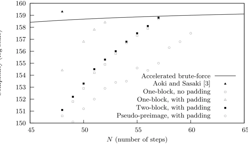
unpractically long messages. No progress has been made since 2009. Our results improve the existing results in several directions: variants with more steps can be attacked, significantly lower complexities are obtained for previously attacked variants, and correctly padded (short!) messages can be computed. The results are summarized in Table 1 and illustrated in Fig. 4 at the end of the paper.

Table 1. Preimage attacks against reduced SHA-1. If not stated otherwise, proper preimages with a correct padding are computed.

Steps Complexity # Blocks Reference Remark

44 2157.0 1 [5]

48 2156.9 1 [3] pseudo-preimage, no padding

48 2159.3 2 [3] no padding

44 2146.2 1 Section 3.2 no padding

48 2150.6 1 ” ”

56 2157.9 1 ” ”

57 2158.7 1 ” ”

48 2149.2 1 Section 3.3 pseudo-preimage

59 2156.8 1 ” ”

60 2157.5 1 ” ”

48 2151.1 2 Section 3.4

56 2158.1 2 ”

57 2158.8 2 ”

Organization. Section 2 describes the new differential perspective on the meet-in-the-middle attack. Section 3 applies the framework to SHA-1 leading to var-ious improved results. Section 4 briefly discusses a slight optimization of the generic brute-force search which can serve as a minimal benchmark for actual attacks. Section 5 summarizes and concludes the paper.

2 Meet-in-the-Middle: A Differential Framework

(4)

2.1 Differential View on the Meet-in-the-Middle Technique

We now describe our new interpretation of the meet-in-the-middle technique. First, F is divided into two parts, F = F2◦F1. Then, from a differential point of view, the attacker tries to find two linear spaces D1, D2 _{⊂ {}0,1_}κ as follows:

– D1∩D2 ={0}.

– For each δ1_∈D1 there is a ∆1 _{∈ {}0,1_}n _{such that}

Pr[∆1=F1(M, P)⊕F1(M ⊕δ1, P)] = 1 (1) for uniformly chosenM, that is, (δ1,0)→∆1 is a related-key differential for F1 with probability 1.

– For each δ2∈D2 there is a ∆2 ∈ {0,1}n such that

Pr[∆2 =F₂−1(M, C)_⊕F₂−1(M _⊕δ2, C)] = 1 (2) for uniformly chosenM, that is, (δ2,0)→∆2 is a related-key differential for F₂−1 with probability 1.

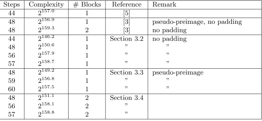
The first condition makes sure that the search space can be partitioned into affine sets of the form M _⊕D1 _⊕ D2. If D1 and D2 both have dimension d these sets contain 22d different messages. Each such set can be searched for a preimage by computing 2d times F1 and 2d times F₂−1 using Algorithm 1. The algorithm computes two listsL1 andL2. A match between the two lists identifies a preimage. The case d= 1 is illustrated by Fig. 1.

The second and the third condition make sure that the algorithm always answers correctly. Using (1) and (2) it follows that L1[δ2] = L2[δ1] (in the last loop of Algorithm 1) is equivalent toF1(M_⊕δ1_⊕δ2, P) =F₂−1(M_⊕δ1_⊕δ2, C), which is true if and only ifM ⊕δ1⊕δ2 is a preimage.

Algorithm 1 Testing M _⊕D1_⊕D2 for a preimage Input: D1, D2 ⊂ {0,1}κ, M ∈ {0,1}κ

Output: A preimage if one is contained in M _⊕D1⊕D2.

for all δ2 ∈D2 do

Compute L1[δ2] =F1(M ⊕δ2, P)⊕∆2.

end for

Compute L2[δ1] =F₂−1(M ⊕δ1, C)⊕∆1.

end for

for all (δ1, δ2)∈D1×D2 do

if L1[δ2] =L2[δ1] then

return M_⊕δ1⊕δ2

end if end for

(5)

P C

L1 L2

F1

M ⊕δ2 ∆2 ∆1

F2

M⊕δ1

F1

M 0 0

F2

M

Fig. 1.Illustration of the meet-in-the-middle attack: A match between the listsL1 and

L2 identifies a preimage. Here, the D1 and D2 only have dimension 1 which allows to test four messages at the cost of two. In general, 22d messages are tested at the cost of 2d, where d is the dimension of D1 and D2.

Complexity Analysis. Algorithm 1 has to be repeated 2n−2d times in order to test 2n _{messages. If we denote by}_Γ1 _and _Γ2 _{the cost of one evaluation of}_F1 _and F2, respectively, this results in a total complexity of 2n−2d(2dΓ1+2dΓ2) = 2n−dΓ, whereΓ is the cost of F. Depending on the implementation, memory is required to store the list L1 and/or L2. Both lists have length 2d _{and entries of about} n+d bits.

Remark. Using non-zero output differences ∆1 and ∆2 corresponds to the idea of indirect matching, introduced in [1], which is a rather advanced matching technique in the Aoki-Sasaki framework. From a differential point of view it appears quite natural.

2.2 Using Probabilistic and Truncated Differentials

Advanced matching techniques such as partial matching [2], indirect partial matching [1], partial fixing [1], and variants of probabilistic matching [10, 20] have a straightforward interpretation in terms of differentials. The conditions on the related-key differentials (δi,0)_→ ∆i are relaxed. Instead of differentials with probability 1 on the full state, probabilistic differentials with truncated output differences can be considered. Truncated differentials go back to Knudsen [11].

For a truncation mask T _{∈ {}0,1_}n _{we denote by =}

T equality on those bits of T which are 1, that is,A =T B if and only if A∧T =B∧T, where ∧is denotes bitwise AND. Instead of (1) and (2), the following probabilities should be high (but can be smaller than 1):

(6)

The only thing that has to be changed in Algorithm 1 is in the last loop, where = has to be replaced with =T. However, the answer of the algorithm is not always correct when using probabilistic and/or truncated differentials which has consequences on the complexity of the attack.

Complexity Analysis. Testing a messageM ⊕δ1⊕δ2 by the modified variant of Algorithm 1 is best formulated as a hypothesis test with null hypothesis

H0: M _⊕δ1_⊕δ2 is a preimage.

H0 is rejected if F1(M _⊕δ2, P) _⊕∆2 ₆=T F₂−1(M ⊕δ1, C) ⊕∆1. H0 is falsely rejected with probability α = 1−p1p2 (type I error probability). On the other hand, if H0 is false, we fail to reject it with probability β = 1/r (type II error probability), where r is the Hamming weight of T. As a consequence, returned messages are only candidate preimages which have to be retested and the total number of tested messages has to be increased. If α is the average type I error probability over all (δ1, δ2) _∈ D1_×D2, 2n_/₍₁₋_α_{) messages have to be tested} in order to compensate a fraction of α preimages that is falsely rejected. This results in a total complexity of

(2n−dΓ + 2n−rΓre)/(1−α),

where Γre is the cost of retesting a candidate preimage.

2.3 Splice and Cut

The splice and cut technique has been first used in [2]. The idea is to start the computations at an intermediate state, connecting the last and the first step via the feed-forward of the Davies-Meyer mode. The technique is fully compatible with our differential framework. Formally, the computation of F is cut into F = F2 ◦ F1 and, for a given target value H, a new function F′ is defined by F′(M, V) = F1(M, H −F2(M, V)). Then, the meet-in-the-middle technique is used to find M such that F′(M, V) = V for some V. This is equivalent to F(M, H −F2(M, V)) + H −F2(M, V) = H, that is, M is a pseudo-preimage. Typically, the pseudo-preimage attack is then generically transformed into a preimage attack as described in [14, Fact 9.99].

2.4 Bicliques

(7)

are lists of 2d states Qi[δ], for δ ∈ Di, such that for all (δ1, δ2) ∈ D1 ×D2: Q2[δ2] = F3(M_⊕δ1_⊕δ2, Q1[δ1]). With such a biclique, the set M_⊕D1_⊕D2 can be searched for candidate pseudo-preimages by testingF1(M⊕δ2, H−Q2[δ2])⊕ ∆2 =T F2−1(M ⊕δ1, Q1[δ1])⊕ ∆1. This requires only 2d computations of F1 and 2d _{computations of} _F2_{. If the amortized cost of constructing many bicliques} is negligible, the number of attacked rounds is increased by the rounds of F3 without actually increasing the total complexity of the attack.

2.5 Special Case: Linear Message Expansion

The differential view is particularly useful if the underlying block cipher F uses a linear key expansion and relatively small round keys. In the following, suppose that F performs N rounds and that the key expansion can be described by N linear maps ϕi : _{0,1_}κ _{→ {}₀_,₁_}w_{, for 0} _≤ _{i < N}_{, where} _w _{is the size of the} round keys and ϕi(K) is the i-th round key derived from K.

Differences as Kernel Elements. If D1 lies in the kernel of ϕi no differences are introduced at round i. For some k > 0, the attacker can choose D1 as a subspace of Tk_i=0−1ker(ϕi). This makes that no differences are introduced in the firstk rounds. Similar,D2 can be chosen as a subspace ofTN_i=N−1₋_kker(ϕi). Then, 2k rounds can be attacked without advanced matching techniques. By a careful choice of D1 and D2 the attack extends to more rounds by using probabilistic and truncated differentials. The kernels can be computed by linear algebra or, as in the case of SHA-1, by using the message expansion in forward and backward direction.

Remark. In [3] kernels of message expansion have been used already. The ker-nel elements have not been interpreted as differences, but a sophisticated linear transformation matrix has been used to derive a “chunk separation” and “neu-tral words”. To make this possible, the condition has been imposed that kernel elements for the two chunks must not have overlapping non-zero words. From a differential point of view it is clear that only D1∩D2 = {0} is required which gives us more freedom in the choice of the attack parameters.

3 Application to SHA-1

We now apply the attack framework to SHA-1, which leads to various new results. Different types of “preimages” will be obtained:

(8)

One-block pseudo-preimages A pseudo-preimage is a “preimage” that uses an incorrect IV. The additional freedom degree allows to use bicliques and the splice and cut technique. This results in pseudo-preimage attacks up to 60 steps. A careful choice of the biclique position avoids additional restrictions from the padding rule such that all our attacks allow to put a correct padding to the pseudo-preimage.

Two-block preimages Combining the above techniques enables us to compute two-block preimages with a correct padding almost as efficiently as one-block preimages without padding. As a result, we obtain preimage attacks up to 57 steps finding correctly padded two-block preimages.

Before describing the attacks, a short description of SHA-1 is given.

3.1 Description of SHA-1

The hash function SHA-1 was designed by the U.S. National Security Agency and is specified in [15]. The construction follows the Merkle-Damg˚ard principle with a block cipher based compression function in Davies-Meyer mode. A message is padded to a length which is a multiple of 512 bits. This is done by appending a 1, a variable number of 0s, and the length in bits as a 64-bit integer. After the padding, the message is split into 512-bit blocks M = (M0_{, . . . ,} _ML−1_{) which} are iteratively processed according to

H0 = IV, Hl+1 =F(Ml, Hl) +Hl, 0 ≤l < L.

The chaining values Hl consist of five 32-bit words. The last chaining value is the output of the hash function.

The function F can be considered as a block cipher with key length κ= 512 and block length n = 160. The computation of F(Ml, Hl) has two parts: First, the message block of 16 words, denoted by Ml _{= (}_M

0, . . . , M15), is expanded to an extended message of 80 words, denoted by W = (W0, . . . , W79):

Wi =Mi, 0 _≤i_≤15,

Wi = (Wi₋3⊕Wi₋8⊕Wi₋14⊕Wi₋16) ≪1, 16≤i < 80.

(5)

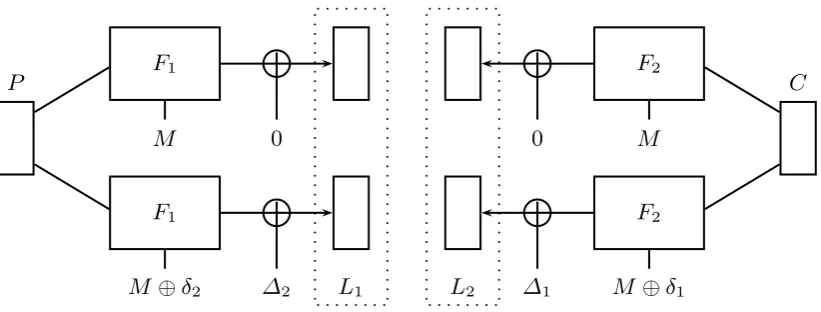
Second, the chaining value Hl _{is loaded into the registers (}_{A, B, C, D, E}_{) and} updated through 80 steps according to Fig. 2. At each step, an expanded message word Wi, a bitwise boolean function fi, and a constant Ki are used. The final content of the registers is the output of F.

3.2 One-Block Preimages

(9)

A B C D E

fj

5

2

Ki Wi

Fig. 2.The step transformation of SHA-1.

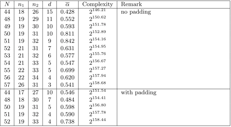
Finding Suitable Attack Parameters. An attack on N steps requires the following parameters: a separation F = F2 ◦ F1 into n1 and n2 = N − n1 steps, two linear spaces D1, D2 _{⊂ {}0,1_}κ _{of dimension} _d_{, output differences} _∆1 (resp. ∆2) for all differences δ1 _∈ D1 (resp. δ2 _∈ D2), and a truncation mask T ∈ {0,1}n _{of Hamming weight} _r_{. The message expansion of SHA-1 is linear} and we can use the techniques from Section 2.5. For 0 _≤ k < 16, the kernel of anyk consecutive steps has dimension (16₋k)_·32. Thus, an attack on 2_·15 = 30 steps is possible without advanced matching techniques. When attacking more steps, (n1−15) : (n2 −15) ≈ 1 : 3 turned out to be a good ratio, because the diffusion is weaker in the backward direction than in the forward direction.

Our main tool for finding attack parameters are two algorithms which allow to experimentally evaluate candidate configurations. Given n1, n2, D1, and D2, the output differences are computed by linearization: ∆1 =F1(δ1,0) and ∆2 = F−₂1(δ2,0), where F1 and F2 are obtained from F1 and F2 by replacing all non-linear Boolean functions fi by (X, Y, Z) 7→ X ⊕Y ⊕Z, replacing + by ⊕, and setting the constants to zero. Then, Algorithm 2 is used to determine a truncation mask T based on a ranking of bitwise difference probabilities, and finally, Algorithm 3 estimates the corresponding type I error probability α. The expected attack complexity is computed as in Section 2.2 withΓre = (N₋30)/N (the first 15 and the last 15 steps don’t have to be recomputed when retesting a candidate preimage).

There is a trade-off between d and α. While this trade-off is hard to analyze by hand, it can be readily explored by our experimental approach. Note that Algorithm 2 always returns a mask of weightr=d. We did not find significantly better attacks for different choices of r. Table 2 summarizes the results for dif-ferent N. All results have been found by extensive experiments using Q = 216 in both algorithms. The full attack parameters are given in the appendix.3

3 _{Note that there is an error in the short version of this paper. The given parameters}

(10)

Algorithm 2 Find truncation mask T for matching Input: D1, D2 ⊂ {0,1}κ

Output: A truncation mask T _{∈ {}0,1_}n of Hamming weight d.

c= an array of ncounters set to 0

forq = 1 toQ do

Choose M _{∈ {}0,1_}κ at random

C _← F(M,IV)

Choose (δ1, δ2)∈D1×D2 at random

∇ ←F1(M⊕δ1,IV)⊕∆1⊕F2−1(M⊕δ2, C)⊕∆2

fori= 0 to n−1 do

if the i-th bit of _∇is 1 then

c[i]_←c[i] + 1

end if end for end for

Set those d bits of T to 1 which have the lowest counters.

Algorithm 3 Estimate type I error probability Input: D1, D2 ⊂ {0,1}κ, T ∈ {0,1}n

Output: Average type I error probability α.

c= a counter set to 0

forq = 1 toQ do

Choose M _{∈ {}0,1_}κ at random

C _← F(M,IV)

Choose (δ1, δ2)∈D1×D2 at random

∇ ←F1(M⊕δ1,IV)⊕∆1⊕F2−1(M⊕δ2, C)⊕∆2

if ∇ 6=T 0n then

c_← c+ 1 // a false rejection of H0

end if end for return c/Q

Attack for N = 57, one-block, no padding. The best result was obtained for a separation into n1 = 26 and n2 = 31 steps, using subspaces D1 and D2 of dimension d = 3. The average type I error probability is estimated as α = 0.541 by Algorithm 3 which results in an expected attack complexity of 2158.68 _{evaluations of the compression function.}

(11)

Table 2. One-block preimages: N is the number of attacked steps, n1 and n2 the number of steps computed by F1 and F2, respectively,d the dimension of D1 and D2, and α the average type I error probability for the filtering of candidate preimages.

N n1 n2 d α Complexity Remark

44 18 26 15 0.428 2146.21 no padding 48 19 29 11 0.552 2150.62

49 19 30 10 0.593 2151.78 50 19 31 10 0.811 2152.89 51 19 32 9 0.842 2154.16 52 21 31 7 0.631 2154.95 53 21 32 6 0.577 2155.76 54 21 33 5 0.547 2156.67 55 22 33 5 0.699 2157.27 56 22 34 4 0.620 2157.94 57 26 31 3 0.541 2158.68

44 17 27 10 0.546 2151.54 with padding 48 18 30 7 0.484 2154.41

50 19 31 5 0.598 2156.80 51 19 32 4 0.590 2157.78 52 19 33 4 0.738 2158.44

3.3 One-Block Pseudo-Preimages

GivenH, we want to findM andH′ such thatH =F(M, H′)+H′. The freedom of choosing H′ allows us to use bicliques and the splice and cut technique.

We separate F into three parts as shown in Fig. 3. The bicliques are con-structed for F3 computing the steps 27−n3 to 26 (n3 steps). F1 computes the steps 27 to 26 +n1 (n1 steps) and F2 computes the steps 27 +n1 to N −1 and 0 to 26₋n3 (n2 steps) using the splice and cut technique. With this choice, the elements of the kernel of the steps 27 to 41 (15 steps) and the elements of the kernel of the steps 11−n3 to 26−n3 (15 steps) automatically satisfy the padding conditions if 0_≤n3 _≤11.

F2

26−n3 27−n3

F3

26 27

F1

26 +n1 27 +n1

F2

Fig. 3.Separation of F for pseudo-preimage attacks. Bicliques are constructed for F3.

(12)

bicliques can be generated from a single one by just modifying some message words outside the biclique. As a result, the amortized cost to construct bicliques is negligible and the complexity computes as 2n−d(Γ1 +Γ2) + 2n−dΓre, where Γ1 +Γ2 = (n1+n2)/N and Γre = (N −n3−30)/N. Table 3 summarizes the results.

Attack for N = 57, pseudo-preimage, with padding. The best result was obtained for a separation into n1 = 19, n2 = 32, and n3 = 6 steps, using subspacesD1 and D2 of dimensiond = 7. The bicliques cover the steps 21 to 26 and for the chosen D1 and D2 (given in the appendix) bicliques with correctly padded messages can be easily found by random search. The average type I error probability is estimated as α = 0.675 which results in an expected attack complexity of 2154.96 evaluations of the compression function.

Table 3. One-block pseudo-preimages: N is the number of attacked steps, n1 and

n2 the number of steps computed by F1 and F2, respectively, n3 is the length of the bicliques, d the dimension of D1 and D2, and α the average type I error probability for the filtering of the candidate preimages.

N n1 n2 n3 d α Complexity Remark

48 18 28 2 12 0.447 2149.22 pseudo-preimage, with padding

49 19 28 2 11 0.398 2150.12

50 19 29 2 10 0.404 2151.15

51 17 30 4 9 0.381 2152.02

52 18 30 4 8 0.332 2152.93

53 18 29 6 7 0.128 2153.46

54 18 30 6 8 0.569 2153.50

55 18 30 7 6 0.208 2154.60

56 19 31 6 8 0.765 2154.41

57 19 32 6 7 0.675 2154.96

58 21 30 7 5 0.478 2156.25

59 19 34 6 5 0.626 2156.78

60 20 34 6 4 0.524 2157.45

3.4 Two-Block Preimages

Given H, we want to find M = (M0, M1) with a correct padding and such thatH =F(M1_{, H}1_{) +}_H1_{, where} _H1 ₌_F₍_M0_,_{IV) + IV). The problem can be} separated into two steps:

1. Find M1 _{such that} _H ₌ _F₍_H1_{, M}1_{) +}_H1 _{for some} _H1 _{and such that} _M1 has a correct padding (a “one-block pseudo-preimage with padding”). 2. For theH1obtained in the first step, findM0such thatH1 =F(M0,IV)+IV

(13)

The two steps can be solved using the attacks from Section 3.2 and 3.3, respec-tively. The total complexity is the sum of both steps, which is dominated by the second step (computing the first block). As an example, forN = 48 we can com-pute a correctly padded two-block preimage with complexity 2150.62+ 2149.22 = 2151.08_{. For} _N _{= 57 the complexity is 2}158.79_.

For N ≥ 58 we lack a method to compute the first block faster than brute-force and we would have to use the generic method from [14, Fact 9.99] to convert a pseudo-preimage attack into a preimage attack. In fact, this is the procedure of most meet-in-the-middle preimage attacks. A pseudo-preimage attack with com-plexity 2m can be converted to a preimage attack with complexity 21+(m+n)/2. In our case, the resulting speed-up is less than a factor two for all results with N _≥58 given in Table 3.

4 Accelerated Brute-Force Search

In this last section we briefly describe a generic optimization of the brute-force search which comes out of the meet-in-the-middle approach. It applies to any number of rounds, but the speed-up is very small. The idea is to not recompute parts of F if they are identical for several messages. This has been previously applied to MD5 [2] and HAVAL-5 [17], and the same idea underlies “matching with precomputation” used for key recovery attacks on AES [4].

Suppose that F can be separated into three parts, F = F2_◦ F3_◦ F1, such that D1 and D2 can be found as in Section 2.1 for F1 and F2, but with zero output differences. Then, Algorithm 4 can be used to test a set M ⊕D1⊕D2. The additional cost compared to Algorithm 1 comes from the 22d _computations ofF3 in the last loop. Testing 2n messages has complexity 2n−d(Γ1+Γ2) + 2nΓ3. Thus, for reasonably large d, the complexity of brute-force search is essentially reduced to 2n _{evaluations of} _F3 _{instead of 2}n _{evaluations of} _F_.

Algorithm 4 Accelerated brute-force search Input: D1, D2 ⊂ {0,1}κ, M ∈ {0,1}κ

Output: A preimage if one is contained in M ⊕D1⊕D2.

Compute L1[δ2] =F1(M ⊕δ2, P).

end for

Compute L2[δ1] =F2−1(M ⊕δ1, C).

end for

for all (δ1, δ2)∈D1×D2 do

if F3(M ⊕δ1⊕δ2, L1[δ2]) =L2[δ1] then

return M_⊕δ1⊕δ2

end if end for

(14)

Application to SHA-1. The speed-up factor is about N/(N −30) for a vari-ant with N steps. Slight improvements are possible by using probabilistic and truncated differentials for F₂−1. For the full SHA-1, a speed-up factor of about two can be obtained. Such an optimization might not be considered as an attack, but it provides a minimal benchmark for actual attacks. Figure 4 compares our results to this benchmark.

5 Summary and Conclusion

We proposed a differential view on the meet-in-the-middle framework originally introduced by Aoki and Sasaki. Advanced matching techniques such as partial matching, indirect partial matching, partial fixing, and probabilistic matching appear very natural from this perspective. For block cipher based hash functions in Davies-Meyer mode, the principal attack parameters are two sets of suitable related-key differentials. Tools are proposed that facilitate a systematic search for these sets.

Applied to SHA-1, our framework leads to significantly better preimage at-tacks up to 57 out of 80 steps. The results are illustrated in Fig. 4 and com-pared to the best previous attack as well as to accelerated brute-force search. The improvements essentially come from a more systematic use of probabilis-tic matching. It is remarkable that we do not rely on the generic conversion of pseudo-preimage attacks into preimage attacks. This allows us to obtain speed-up factors that would be hard to achieve with the generic conversion.

Application of the framework to the SHA-2 family seems more complicated, namely due to the non-linear message expansion. Nevertheless, it is expected that the differential perspective on meet-in-the-middle attacks leads to improved results on other primitives as well.

Acknowledgements. We thank Christian Rechberger for interesting discus-sions on preimage attacks and SHA-1. Many thanks also to Sebastiano Degan for independent verification of our experimental results and for pointing out an error in the attack parameters given in the short version of this paper. This work was partially supported by the Hasler Foundation www.haslerfoundation.ch under project number 08065.

References

1. Aoki, K., Guo, J., Matusiewicz, K., Sasaki, Y., Wang, L.: Preimages for Step-Reduced SHA-2. In: Matsui, M. (ed.) ASIACRYPT. Lecture Notes in Computer Science, vol. 5912, pp. 578–597. Springer (2009)

2. Aoki, K., Sasaki, Y.: Preimage Attacks on One-Block MD4, 63-Step MD5 and More. In: Avanzi, R.M., Keliher, L., Sica, F. (eds.) Selected Areas in Cryptography. Lecture Notes in Computer Science, vol. 5381, pp. 103–119. Springer (2008) 3. Aoki, K., Sasaki, Y.: Meet-in-the-Middle Preimage Attacks Against Reduced

(15)

150 151 152 153 154 155 156 157 158 159 160

45 50 55 60 65

C o m p le xi ty (l o g sc a le )

N (number of steps)

Accelerated brute-force Aoki and Sasaki [3]

u

One-block, no padding

rs rs rs rs rs rs rs rs rs rs rs

One-block, with padding

ut

Two-block, with padding

r r r r r r r r r r r

Pseudo-preimage, with padding

bc bc bc bc bc bc bc bc bc bc bc bc bc

Fig. 4. Preimage attacks against reduced SHA-1: Illustration of the new results and comparison to accelerated brute-force search.

4. Bogdanov, A., Khovratovich, D., Rechberger, C.: Biclique cryptanalysis of the full aes. In: Lee, D.H., Wang, X. (eds.) ASIACRYPT. Lecture Notes in Computer Science, vol. 7073, pp. 344–371. Springer (2011)

5. Canni`ere, C.D., Rechberger, C.: Preimages for Reduced SHA-0 and SHA-1. In: Wagner, D. (ed.) CRYPTO. Lecture Notes in Computer Science, vol. 5157, pp. 179–202. Springer (2008)

6. Chabaud, F., Joux, A.: Differential Collisions in SHA-0. In: Krawczyk, H. (ed.) CRYPTO. Lecture Notes in Computer Science, vol. 1462, pp. 56–71. Springer (1998)

7. Chaum, D., Evertse, J.H.: Crytanalysis of DES with a Reduced Number of Rounds: Sequences of Linear Factors in Block Ciphers. In: Williams, H.C. (ed.) CRYPTO. Lecture Notes in Computer Science, vol. 218, pp. 192–211. Springer (1985)

8. Diffie, W., Hellman, M.: Special Feature Exhaustive Cryptanalysis of the NBS Data Encryption Standard. Computer 10, 74–84 (1977)

9. Guo, J., Ling, S., Rechberger, C., Wang, H.: Advanced Meet-in-the-Middle Preim-age Attacks: First Results on Full Tiger, and Improved Results on MD4 and SHA-2. In: Abe, M. (ed.) ASIACRYPT. Lecture Notes in Computer Science, vol. 6477, pp. 56–75. Springer (2010)

10. Khovratovich, D., Rechberger, C., Savelieva, A.: Bicliques for Preimages: Attacks on Skein-512 and the SHA-2 family. In: Canteaut, A. (ed.) FSE. Lecture Notes in Computer Science, Springer (2012)

11. Knudsen, L.R.: Truncated and Higher Order Differentials. In: Preneel, B. (ed.) FSE. Lecture Notes in Computer Science, vol. 1008, pp. 196–211. Springer (1994) 12. Leurent, G.: MD4 is Not One-Way. In: Nyberg, K. (ed.) FSE. Lecture Notes in

(16)

13. Mendel, F., Pramstaller, N., Rechberger, C., Kontak, M., Szmidt, J.: Cryptanalysis of the GOST Hash Function. In: Wagner, D. (ed.) CRYPTO. Lecture Notes in Computer Science, vol. 5157, pp. 162–178. Springer (2008)

14. Menezes, A.J., van Oorschot, P.C., Vanstone, S.A.: Handbook of Applied Cryp-tography. CRC Press (1996)

15. National Institute of Standards and Technology: FIPS 180-3: Secure Hash Standard (2008), http://www.itl.nist.gov/fipspubs/

16. Sasaki, Y., Aoki, K.: A Preimage Attack for 52-Step HAS-160. In: Lee, P.J., Cheon, J.H. (eds.) ICISC. Lecture Notes in Computer Science, vol. 5461, pp. 302–317. Springer (2008)

17. Sasaki, Y., Aoki, K.: Preimage Attacks on 3, 4, and 5-Pass HAVAL. In: Pieprzyk, J. (ed.) ASIACRYPT. Lecture Notes in Computer Science, vol. 5350, pp. 253–271. Springer (2008)

18. Sasaki, Y., Aoki, K.: Preimage Attacks on Step-Reduced MD5. In: Mu, Y., Susilo, W., Seberry, J. (eds.) ACISP. Lecture Notes in Computer Science, vol. 5107, pp. 282–296. Springer (2008)

19. Sasaki, Y., Aoki, K.: Finding Preimages in Full MD5 Faster Than Exhaustive Search. In: Joux, A. (ed.) EUROCRYPT. Lecture Notes in Computer Science, vol. 5479, pp. 134–152. Springer (2009)

20. Wang, L., Sasaki, Y.: Finding Preimages of Tiger Up to 23 Steps. In: Hong, S., Iwata, T. (eds.) FSE. Lecture Notes in Computer Science, vol. 6147, pp. 116–133. Springer (2010)

(17)

A

Attack Parameters for SHA-1

The attack complexities given in this paper rely on experiments, namely in an estimated value of the average type I error probability α. In the following we provide all the details which are required to reproduce the results.

A.1 Description of Attack Parameters

The attack parameters always include the separation ofF (given by n1 and n2), two linear difference spacesD1 andD2of dimension d, and a truncation maskT. Additionally, when using bicliques and the splice and cut technique, the length of the bicliques is required (given byn3) and a sample biclique is given in order to demonstrate that suitable bicliques indeed exist. We use the following notations and conventions:

– C-style hex notation for 32-bit words: for example 0x5a827999 is the round constant K0 in SHA-1.

– The linear spaces D1 and D2 have a particular form which allows them to be represented by a single element and the dimension d. If the difference x0||. . .||x15 is given, a basis of the corresponding subspace is obtained by word-wise rotation as follows: (x0 ≪i)_||. . ._||(x15 ≪i) for i= 0, . . . , d₋1.

– A biclique is specified by one of its states, say Q1[0], a message M, and the subspacesD1 andD2. The remaining states of the biclique can be computed using the definition (see Section 2.4).

A.2 Parameters for Results in Table 2 (one-block, no padding)

N = 44, n1 = 18, n2 = 26, d = 15

D1: 0x00000000 0x00000000 0x00000000 0x00000000 0x00000000 0x00000000 0x00000000 0x00000000 0x00000000 0x00000000 0x00000000 0x00000000 0x00000000 0x00000000 0x00000000 0x00000008

D2: 0xc0000000 0x00000000 0x80000000 0x80000000 0x40000000 0x00000000 0x80000000 0x80000000 0x40000000 0x00000000 0x00000000 0x80000000 0xc0000000 0x00000000 0x80000000 0x80000000

T: 0xe0000007 0xe0000007 0xc0000001 0x00000000 0x00000000 N = 48, n1 = 19, n2 = 29, d = 11

(18)

N = 49, n1 = 19, n2 = 30, d = 10

T: 0xc0000001 0xc0000005 0x40000001 0x00000001 0x00000000

N = 50, n1 = 19, n2 = 31, d = 10

T: 0xe0000001 0x80000007 0x00000001 0x00000001 0x00000000

N = 51, n1 = 19, n2 = 32, d = 9

T: 0x80000007 0x00000007 0x00000001 0x00000001 0x00000000

N = 52, n1 = 21, n2 = 31, d = 7

D2: 0x40000000 0x00000000 0xa0000000 0x80000000 0xa0000000 0x00000000 0x80000000 0x00000000 0xc0000000 0x00000000 0x80000000 0x80000000 0x40000000 0x00000000 0x80000000 0x80000000

T: 0x40000000 0x00000006 0xc0000001 0x00000001 0x00000000

N = 53, n1 = 21, n2 = 32, d = 6

(19)

T: 0x40000000 0x00000005 0x40000001 0x00000001 0x00000000 N = 54, n1 = 21, n2 = 33, d = 5

T: 0xc0000000 0x00000004 0x00000001 0x00000001 0x00000000 N = 55, n1 = 22, n2 = 33, d = 5

T: 0x00000004 0x80000001 0x00000001 0x00000001 0x00000000 N = 56, n1 = 22, n2 = 34, d = 4

T: 0x00000004 0x80000001 0x00000001 0x00000000 0x00000000 N = 57, n1 = 26, n2 = 31, d = 3

D2: 0x80000000 0x80000000 0x80000000 0x00000000 0x00000000 0x40000000 0x00000000 0xa0000000 0x80000000 0xa0000000 0x00000000 0x80000000 0x00000000 0xc0000000 0x00000000 0x80000000

(20)

A.3 Parameters for Results in Table 2 (one-block, with padding)

N = 44, n1 = 17, n2 = 27, d = 10

D2: 0x00000004 0x00000014 0x00000000 0x00000000 0x00000004 0x0000001c 0x00000010 0x00000000 0x00000004 0x0000001c 0x00000008 0x00000018 0x0000000c 0x00000004 0x00000000 0x00000000

T: 0x0000003c 0x0000003c 0x00000006 0x00000000 0x00000000 N = 48, n1 = 18, n2 = 30, d = 7

T: 0x00000018 0x0000001c 0x00000006 0x00000000 0x00000000 N = 50, n1 = 19, n2 = 31, d = 5

D2: 0x80000003 0x40000002 0x60000002 0xc0000001 0xa0000003 0x00000001 0x00000002 0x80000001 0xc0000003 0x00000002 0x00000000 0x00000000 0x40000003 0x00000002 0x00000000 0x00000000

T: 0x00000007 0x00000000 0x80000001 0x00000000 0x00000000 N = 51, n1 = 19, n2 = 32, d = 4

D2: 0x08000000 0x18000000 0x04000000 0x1a000000 0x0c000000 0x0e000000 0x10000000 0x00000000 0x18000000 0x04000000 0x00000000 0x00000000 0x10000000 0x1c000000 0x00000000 0x00000000

T: 0x38000000 0x20000000 0x00000000 0x00000000 0x00000000 N = 52, n1 = 19, n2 = 33, d = 4

(21)

D2: 0x04000000 0x04000000 0x02000000 0x02000000 0x16000000 0x1a000000 0x1c000000 0x08000000 0x1c000000 0x0c000000 0x10000000 0x00000000 0x1c000000 0x14000000 0x00000000 0x00000000

T: 0x78000000 0x00000000 0x00000000 0x00000000 0x00000000

A.4 Parameters for Results in Table 3 (pseudo, with padding)

N = 48, n1 = 18, n2 = 28, n3 = 2,d = 12

T: 0x0000007c 0x00000078 0x00000018 0x00000010 0x00000000 Q1[0]: 0x9ee4eb7b 0xfaf60c40 0x3d9f5367 0x4faed2df 0x102cdff0

M: 0x1e45706f 0x23072fb4 0x83ca0391 0xd019a507 0xfaf436fe 0xf1a5323a 0xd5b723dc 0xe3ab26bc 0x60d820ff 0x823704a1 0x52a9a83b 0xd251e88b 0x5efac42d 0xa156a969 0x00000000 0x000003bf

N = 49, n1 = 19, n2 = 28, n3 = 2,d = 11

T: 0x00000018 0x0000007c 0x0000001c 0x00000010 0x00000000 Q1[0]: 0xa1dc712e 0x95d62d62 0x92df251f 0x7bcbb2c6 0x2fe93f9b

M: 0xfc9adc5d 0x3e808f27 0x88c2d680 0x8d1369d6 0x344e2afa 0x3b33e529 0x274bffd3 0x88209079 0x4f2d897d 0x3b56b074 0x95135463 0xed2aa206 0x2e889c55 0xcba1d561 0x00000000 0x000003bf

N = 50, n1 = 19, n2 = 29, n3 = 2,d = 10

(22)

Q1[0]: 0xdf32bba1 0xec891b4d 0x187d32d3 0xf4393c27 0x46b65b83

M: 0xafe5cd01 0xca7ff558 0x2b762e13 0x3b5ac985 0x76cc73cf 0x435e511b 0xb97d9f39 0xecb73848 0x2c594bfd 0x39f075e6 0x891cf868 0x8e5fd6a3 0x4aceb64c 0x54132315 0x00000000 0x000003bf

N = 51, n1 = 17, n2 = 30, n3 = 4,d = 9

T: 0x0000003c 0x0000007c 0x00000000 0x00000000 0x00000000 Q1[0]: 0x1fb4844b 0xc4eb4d4c 0xffccc87a 0x74f112bd 0xb33d94f1

M: 0x3b2701c3 0x532837db 0xeff9477f 0x4f8ab29f 0xf05433ee 0xebad6bc4 0x1b9933e5 0xf07f0a3d 0x536d687b 0x315d017c 0x87bb41d2 0xd7cf7647 0x8fe9fffa 0x4f9a2687 0x00000000 0x000003bf

N = 52, n1 = 18, n2 = 30, n3 = 4,d = 8

T: 0x0000001c 0x0000003c 0x00000004 0x00000000 0x00000000 Q1[0]: 0xf6b1c9fd 0x0e30107b 0x9308c95d 0xc955f6e3 0x656e0e53

M: 0x18d3ab4b 0xf0e83376 0x80a8fa1a 0x286eaa4c 0xe947fef2 0x3a974781 0x99f70ef6 0x339ad3c3 0xae688d27 0xe5f6533b 0x3e9e7eca 0xa5a21b0c 0x24b2b404 0x2373a2d7 0x00000000 0x000003bf

N = 53, n1 = 18, n2 = 29, n3 = 6,d = 7

D1: 0x00800000 0x00800000 0x00400000 0x00000000 0x00800000 0x00800000 0x00400000 0x00000000 0x00000000 0x00800000 0x00c00000 0x00000000 0x00800000 0x00800000 0x00000000 0x00000000

(23)

M: 0x9c34e7cf 0x88c0c05b 0xf004c8ed 0xe80233b3 0xfd105a66 0x846f1ff3 0xf948b1ee 0xd43fa31e 0x35dd01db 0x38e640bf 0x4cd2dd3e 0xff42a038 0xd64f98d3 0x734e7feb 0x00000000 0x000003bf

N = 54, n1 = 18, n2 = 30, n3 = 6,d = 8

T: 0x00000001 0x00000010 0x0000000f 0x0000000c 0x00000000 Q1[0]: 0x7d3eebf0 0xf8c333c5 0xce413a03 0xbb70c7c5 0x8f1034a9

M: 0x32fb067d 0x54eb75ba 0xdbe304c3 0x2389c4bc 0x679195c1 0x188df1ff 0x5aca2211 0x36ed7d12 0x34ee1e98 0x5f07d210 0x28a18e32 0x1ccb6315 0x139d4efd 0x888124e7 0x00000000 0x000003bf

N = 55, n1 = 18, n2 = 30, n3 = 7,d = 6

T: 0x00000007 0x00000000 0x80000003 0x00000000 0x00000000 Q1[0]: 0x67d71ad3 0xd421573b 0x06575daa 0x32448a3a 0x290c7720

M: 0xf695e1ae 0x21db1192 0x248c67ba 0x13349385 0x90f957c5 0x9f48780f 0xa0574385 0x4c6a7df4 0x75dc07e0 0x14ec69fe 0xa429bebc 0x61c7b895 0x21b1114a 0xa7c8eb73 0x00000000 0x000003bf

N = 56, n1 = 19, n2 = 31, n3 = 6,d = 8

(24)

M: 0xdc467f36 0xa7de388e 0x96ff6b6f 0x83a9070d 0xb96959e7 0xef872e08 0xc985d88e 0x6faa299e 0xb41b3686 0xc1635fbc 0xb6dd33ae 0x4f10520b 0x7100ff03 0x9fe99105 0x00000000 0x000003bf

N = 57, n1 = 19, n2 = 32, n3 = 6,d = 7

T: 0x00000003 0x00000000 0x80000003 0x00000003 0x00000000 Q1[0]: 0x1c2652fe 0x53eb4c0a 0x57e9168f 0xf65b3a56 0x7c428e01

M: 0xce369809 0x3ea1797b 0x1ab39a0d 0x96d1d5e0 0x7a550f31 0xad4da4dd 0x0f72712f 0x17d8a5e8 0xdad6d21d 0x3b0faf80 0x7cc259ff 0xb27a9d25 0x22a02a94 0x88bbfd35 0x00000000 0x000003bf

N = 58, n1 = 21, n2 = 30, n3 = 7,d = 5

T: 0x00000000 0x00000000 0x00000000 0xf0000001 0x00000000 Q1[0]: 0x77f88fc0 0xef5f9fab 0xa53354bc 0x7ebfcd0f 0xe9bdf64c

M: 0x9c8db6ac 0xf00b105f 0x9bc20b30 0xd61c24b4 0xb7c07ff0 0xf0715fbb 0xabc44099 0x2d29be5a 0x0a49f67b 0x7befcf1b 0xc8b7bbd6 0x9800488d 0xf49d23e2 0x423af681 0x00000000 0x000003bf

N = 59, n1 = 19, n2 = 34, n3 = 6,d = 5

(25)

M: 0xff725191 0xf85050c3 0x6076def2 0x8e86d6c2 0x158d7a79 0x6220da96 0x998f05a6 0xc0a7591a 0xfeaafdec 0xd0ef7a21 0x3cc64d89 0x55b76464 0x5e0611c2 0xc226ac03 0x00000000 0x000003bf

N = 60, n1 = 20, n2 = 34, n3 = 6,d = 4

T: 0x0000003c 0x00000000 0x00000000 0x00000000 0x00000000 Q1[0]: 0x1cea526c 0xeecf2c58 0xdb83824f 0x0383abe3 0xa00c961e