using
η
TPairing
Naoyuki Shinohara1, Takeshi Shimoyama2, Takuya Hayashi3, and Tsuyoshi Takagi3
1
National Institute of Information and Communications Technology,
2 FUJITSU LABORATORIES Ltd., 3
Kyushu University.
Abstract. The security of pairing-based cryptosystems depends on the difficulty of the discrete logarithm problem (DLP) over certain types of finite fields. One of the most efficient algorithms for computing a pairing is the ηT pairing over supersingular curves on finite fields whose characteristic is 3. Indeed many high-speed implementations of this pairing have been reported, and it is an attractive candidate for practical deployment of pairing-based cryptosystems. The embedding degree of theηT pairing is 6, so we deal with the difficulty of a DLP over the finite field GF(36n), where the function field sieve (FFS) is known as the asymptotically fastest algorithm of solving it. Moreover, several efficient algorithms are employed for implementation of the FFS, such as the large prime variation. In this paper, we estimate the time complexity of solving the DLP for the extension degreesn= 97,163,193,239,313,353,509, when we use the improved FFS. To accomplish our aim, we present several new computable estimation formulas to compute the explicit number of special polynomials used in the improved FFS. Our estimation contributes to the evaluation for the key length of pairing-based cryptosystems using theηT pairing.
Keywords: pairing-based cryptosystems, discrete logarithm problem, finite field, key length, suitable values
1 Introduction
Pairing-based cryptosystems such as identity-based encryption [9] have recently become one of the main research topics in cryptography. Their security is based on the intractability of the discrete logarithm problem (DLP) over certain types of finite fields. Once the underlying DLP is broken, the pairing-based cryptosystems are no longer secure. Therefore, evaluating the intractability of a DLP is an important task.
One of the most efficient algorithms for computing a pairing is the ηT pairing defined over
su-persingular curves on finite fields whose characteristic is 3 [7]. Many high-speed implementations of theηT pairing have been reported in previous literature [4, 8, 15, 16, 22], and there are many efficient
algorithms for Tate pairing over finite fields whose characteristic is 3 [6, 11, 12, 17, 24, 28]. The timings reported in the literature are appealing for using theηT pairing in practices; therefore in this paper we
deal with the DLP over finite fields whose characteristic is 3. Moreover, since the embedding degree of the ηT pairing is 6, we are interested in finite fields GF(36n) for some integersn.
In this paper, we try to estimate the time complexity of solving the DLP overGF(36n) for extension
degreesn= 97, 163, 193, 239, 313, 353, 509, using the following background facts. In 2010, Hayashi et al. solved a 676-bit DLP (overGF(36·71)) [18]. Joux and Lercier estimated that the time complexity of solving the DLP overGF(36·97) is around 271 [21]. And Smart et al. showed that the difficulty of
solving the DLP overGF(36·193) is roughly equivalent to that of factoring a 1024-bit RSA key (80-bit security) [30]. NIST recommended using a key size of more than 80 bits after 2011 [5]. Ahmadi et al. assumed that the DLP with n= 509 has the security level of 128 bits [4].
To estimate the time complexity, we consider an efficient algorithm to solve a DLP over GF(36n). Adleman proposed the function field sieve (FFS) to practically solve a DLP over finite fields whose characteristic is small [1, 3]. The time complexity of the FFS for a DLP overGF(36n) is asymptotically
Table 1.Estimation of the time complexity of solving DLP overGF(36n)
n 97 163 193 239 313 353 509 log2Csieve52.79 68.17 71.90 78.08 90.04 94.42 111.35
n: extension degree of the fieldGF(36n) over its base fieldGF(36).
Csieve: computational cost of the sieving step of the improved FFS (In this paper, we ultimately regardCsieveas the time complexity of solving the DLP overGF(36n).)
forn→ ∞. In 2002, Joux and Lercier proposed a practical improvement of the FFS called JL02-FFS [20], and in 2006 another new variant of the FFS (JL06-FFS) for GF(q), where the characteristic is small and q is a medium-sized prime power [21]. Hayashi et al. reported that JL06-FFS has an advantage over JL02-FFS when we try to solve a DLP overGF(36n) [18]. Additionally, there are well-known efficient algorithms for implementation of JL06-FFS: the large prime variation [26], lattice sieve [27], filtering [10], Galois action [18] and free-relation [18]. Thus, we estimate the time complexity of solving a overGF(36n) by JL06-FFS with these efficient algorithms. We call this FFS “the improved FFS” in this paper.
There is an elemental parameter (κ, dH, dm, B, R, S) commonly-utilize in JL06-FFS (FFS) and
the improved FFS. There is also an advanced parameter (λ, θ, β) for the improved FFS, where λ is for the large prime variation, θ for the lattice sieve, and β for the filtering. For our estimation of the time complexity, we require the value of the parameter (κ, dH, dm, B, R, S, λ, θ, β), such that the
computational cost of the improved FFS is almost minimum, when the extension degreesnare fixed. In this paper, such values are called the “suitable values” of (κ, dH, dm, B, R,
S, λ, θ, β). To find suitable values for the fixed extension degrees n, we performed an experiment via a personal computer with an Intel Quad-Core (2.8 GHz) CPU and 8 GB RAM, and it took roughly 57 hours. Specifically, we checked certain computable criteria to solve a DLP with the improved FFS, changing the values of (κ, dH, dm, B, R, S, λ, θ, β). The criteria are checkable by using our new
formulas (22), etc., which are extended from Granger’s formula [13]. (Section 5 provides details on our experiment.)
Through the experiment we obtained Table 3 of the suitable values, and were able to eventually regard the computational costCsieve of the sieving step of the improved FFS as the time complexity
of solving the DLP overGF(36n). On the strength of the costsC
sieve, we present Table 1 of the time
complexity estimation of solving the DLP overGF(36n).
The hardness of the DLP over GF(36·509) was estimated to be equivalent to 128-bit security [4], however, the DLP overGF(36·509) actually accomplishes only about 111-bit security. To safely utilize a cryptographic schemes withηT pairing overGF(3n), we must be aware of this fact.
2 Outline of function field sieve
2.1 DLP and ηT pairing
We first refer to a discrete logarithm (DLP) over the multiplicative group GF(36n)∗. Let g be a generator of the multiplicative groupGF(36n)∗ and A∈ hgi. We then try to solve the DLP over hgi; namely, we compute the smallest positive integer loggA such thatgloggA=A.
It is expected that theηT paring over the supersingular curve onGF(3n) realizes practical
pairing-based cryptosystems. The safety of these cryptosystems is pairing-based on the difficulty of the DLP over
GF(36n), since the map η
T is a bilinear map from G1 × G2 to GF(36n), where G1 and G2 are
cyclic groups. For example, let α be a secret integer such that v1 = [α]v2 for given v1, v2 ∈ G1. We
then prepare arbitraryw ∈G2 and compute ηT(v1, w), ηT(v2, w). Since ηT(v1, w) = ηT([α]v2, w) = ηT(v2, w)α∈GF(36n)∗, we can obtainα by solving the DLP overGF(36n)∗.
2.2 FFS
There are several variants of FFS. Adleman proposed the first FFS in 1994 [1], and Adleman and Huang later proposed a practical FFS [3]. Joux and Lercier proposed two more practical FFS’s; JL02-FFS [20] and JL06-JL02-FFS [21]. Hayashi et al. reported that JL06-JL02-FFS has an advantage over JL02-JL02-FFS in solving a DLP overGF(36n) [18], so we introduce JL06-FFS. From this section, FFS means JL06-FFS. We begin with an overview of the FFS, and suppose that we try to obtain loggA in this section. This consists of four steps: polynomial selection, sieving, linear algebra, and individual logarithm. The parameter (κ, dH, dm, B, R, S) of FFS is called the elemental parameter of the FFS.
Polynomial selection : Let κ be the extension degree of the coefficient field of GF(3κ)[x], where κ= 1,2,3,6. We select a monic irreducible polynomial f ∈GF(3κ)[x], a polynomialm∈GF(3κ)[x], and a bivariate polynomial H(x, y) =x+ydH ∈GF(3κ)[x, y] such that
H(x, m)≡0 (mod f), degf = 6n/κ. (1)
Note that, by lettingdm be degm, the following property holds:
dm·dH ≥degf. (2)
Then the finite fieldGF(36n) is described asGF(3κ)[x]/(f). AndH(x, y) satisfies the eight conditions proposed by Adleman [1]. There is a surjective homomorphism
Φ: {
GF(3κ)[x, y]/(H) → GF(36n)∼=GF(3κ)[x]/(f)
y 7→ m.
Here we select the smoothness boundB and define a rational factor base ¯F(B) and an algebraic factor base ˆF(B) as follows:
¯
F(B) ={p∈GF(3κ)[x]| deg(p)≤B, pis irreducible},
ˆ
F(B) ={hp, y−ti ∈Div(GF(3κ)[x, y]/(H))|p∈F¯(B), t≡m (mod p)},
where Div(GF(3κ)[x, y]/(H)) is the divisor group of GF(3κ)[x, y]/(H) and hp, y −ti is a divisor generated byp and y−t.
Sieving: For given positive integersR, S, we find pairs (r, s)∈(GF(3κ)[x])2 such that
degr≤R,degs≤S,gcd(r, s) = 1, r is monic, (3)
rm+s= ∏
pi∈F¯(B)
pai
i (4)
hry+si= ∑
hpj,y−tji∈Fˆ(B)
by a sieving algorithm. The property (5) can be translated into the following equation:
(−r)dHH(x, −s/r) = (−r)dHx+sdH = ∏ hpj,y−tji∈F(B)ˆ
pbj
j . (6)
Thus, in particular, we collect (r, s) satisfying (3), (4) and (6). And such (r, s) is called a B-smooth pair. Let h be the class number of the quotient field of GF(3κ)(x)[y]/(H), and we assume that h is coprime to (36n−1)/(3κ−1). Finally, we obtain the following congruent:
∑
pi∈F(B)¯
ailoggpi ≡
∑
hpj,y−tji∈F(B)ˆ
bjloggκj (mod (36n−1)/(3κ−1)), (7)
where κj =Φ(λj)1/h, hλji =hhpj, y−tji. The congruent (7) is called arelation. LetRsieve be the
number of relations obtained in the sieving step, and then we require the following criteria that
Rsieve≥(# ¯F(B) + # ˆF(B)). (8)
Linear algebra: After generating a linear equation from relations, we translate it into a smaller linear equation by an algorithm such as the filtering. The smaller one is solved via an algorithm such as the Lanczos method [2, 25], and then we obtain
loggp1, ...,loggp# ¯F(B),loggκ1, ...,loggκ# ˆF(B).
Individual logarithm: Using the special-Q descent method [21], we compute integers ei, fj such
that
loggA≡ ∑ pi∈F¯(B)
eiloggpi+
∑
hpj,y−tji∈Fˆ(B)
fjloggκj (mod (36n−1)/(3κ−1))
Then we obtain the discrete logarithm loggA.
3 Known evaluation methods
The computational cost of FFS is greatly influenced by the parameter selection of the FFS. For example, if we add only 1 to the value of the parameter R of the FFS given in equation (3), the computational cost of sieving increases 3κ-fold. Therefore, the value of the parameter of the FFS must be meticulously selected.
The elemental parameter (κ, dH, dm, B, R, S) of the FFS is given in section 2.2. For a fixed pair
3.1 Asymptotic evaluation formulas
From asymptotic analysis in [21], when we solve a DLP over a finite field GF(3κ)[x]/(f) for given
integersκ,degf by FFS, the smallest positive integer satisfying (9) is generally selected as the value ofB:
(B+ 1) log 3κ≥ √
degf B log
degf
B . (9)
We then assume thatR=S=B and
dH =
l√
degf /B
m
. (10)
We also calculate the smallest integer dm satisfying (2) for the given dH and degf. We then have
Table 2 of approximate suitable values of the elemental parameter of FFS.
Table 2.Approximate suitable values of elemental parameter of FFS
n 97 163 193 239 313 353 509
κ 1 2 3 6 1 2 3 6 1 2 3 6 1 2 3 6 1 2 3 6 1 2 3 6 1 2 3 6 dH 6 6 6 6 7 7 7 7 7 7 7 7 8 8 8 8 8 8 8 8 9 9 9 9 10 10 10 10 dm97 49 33 17 140 70 47 24 166 83 56 28 180 90 60 30 235 118 79 40 236 118 79 40 306 153 102 51 B 18 9 6 3 23 11 7 4 24 12 8 4 27 13 9 4 30 15 10 5 31 16 10 5 37 18 12 6 R 18 9 6 3 23 11 7 4 24 12 8 4 27 13 9 4 30 15 10 5 31 16 10 5 37 18 12 6 S 18 9 6 3 23 11 7 4 24 12 8 4 27 13 9 4 30 15 10 5 31 16 10 5 37 18 12 6
n: extension degree of the fieldGF(36n) over its base fieldGF(36)
κ: extension degree of the coefficient field ofGF(3κ)[x] such thatGF(36n)'GF(3κ)[x]/(f), wheref∈GF(3κ)[x] is a monic irreducible polynomial of degree 6n/κ
dH: degree inyof the bivariate polynomialH(x, y) =x+ydH ∈GF(3κ)[x, y] used for FFS dm: degree of the polynomialminGF(3κ)[x] such thatH(x, m)≡0 (modf)
B: smoothness bound for FFS
R: maximum degree of polynomialr∈GF(3κ)[x] used in the sieving step of FFS S: maximum degree of polynomials∈GF(3κ)[x] used in the sieving step of FFS
3.2 Granger’s evaluation formula
Granger proposed a sharp evaluation formula in (15) to estimate the running time of FFS. By extending
ρ1 in (15) we obtain our new functions ρ2 and ρ3 in section 4.3. Here we briefly explain Granger’s
method, and more detail is given in [13].
There is a problem about deciding on the smoothness bound B of factor bases ¯F(B) and ˆF(B). The numbers of factor bases increase exponentially, and take discrete values sinceB is an integer. To correct this problem, Granger naturally extends B-smooth to (B, β)-smooth with a new parameter
β ∈(0,1]. The new parameter β means the ratio of the number of polynomials in ¯F(B) of degreeB
to that of all monic irreducible polynomials inGF(3κ)[x] of degree B.
In fact, factor bases ¯F(B) and ˆF(B) are extended to ¯F(B, β) and ¯F(B, β) such that
¯
F(B, β) = ¯ΛtF¯(B−1),Fˆ(B, β) = ˆΛtFˆ(B−1),
factor ofgis in the factor base ¯F(B, β). In the same manner as the rational side, (B, β)-smooth is also introduced in the algebraic side. Therefore, B-smooth pair in section 2.2 can be naturally extended to (B, β)-smooth pair. In fact, a pair (r, s) is said to be a (B, β)-smooth pair if the (r, s) satisfies (3) and the following properties that
rm+s= ∏
pi∈F(B¯ −1)
pai
i
∏
Pj∈Λ¯
Baj
j , (11)
(−r)dHx+sdH = ∏ hpi,y−tii∈Fˆ(B−1)
pbi
i
∏
hPj,y−tji∈Λˆ
Bbj
j , (12)
which correspond to (4) and (6) respectively. The criteria (8) is described as
Rsieve≥2# ¯F(B, β), (13)
since ¯F(B, β) and ˆF(B, β) have almost the same cardinality in practice. For checking this criteria, Granger proposed two formulas to compute Rsieve and # ¯F(B, β). First, we discuss how to compute
# ¯F(B, β). Let Iq(k) be the number of monic irreducible polynomials in GF(q) of degree k. Iq(k) is
computable by the equationIq(k) = 1k
∑
d|kµ(d)qk/d, whereµ is themobius function. We then have
the following formula:
# ¯F(B, β) =
B∑−1
k=1
Iq(k) +bβIq(B)c. (14)
Next we consider Rsieve, namely the number of (B, β)-smooth pairs (r, s) collected in the sieving
step. Letρ1(q, B, β, k) be the probability that a monic polynomial in GF(q)[x] of degree kis (B, β
)-smooth. For given non-negative integersi, j, let ¯ai,j be the number of pairs (r, s) satisfying (3). We
denoteDN R(i, j), DN A(i, j) by the degrees ofrm+sand (−r)dHx+sdH respectively, wherei= degr
and j= degs. Then Rsieve is described as
R
∑
i=0 S
∑
j=0
ρ1(q, B, β, DN R(i, j))ρ1(q, B, β, DN A(i, j))¯ai,j, (15)
and the function ¯ai,j is given in Appendix A.
4 New evaluation formulas for efficient implementation of FFS
To solve the DLP overGF(36n) forn≥97, we employ several efficient algorithms for implementation
of the FFS; large prime variation [26], lattice sieve [27], filtering [10], Galois action [18], and free relation [18]. These algorithms are not considered in Granger’s method. Especially, for lattice sieve and large prime variation, new parametersθ andλare respectively introduced. We extend Granger’s formula for the FFS with those efficient algorithms. (We call this FFS the “improved FFS.”) Then the number Rsieve of the relations given by the sieving step of the improved FFS is computable by
exchangingρ1 in (15) with our new formulasρ2 andρ3 in section 4.3. As mentioned in section 3.2, we
also suppose that ¯F(B, β) and ˆF(B, β) have almost the same cardinality in this section.
4.1 Well-used efficient algorithms for FFS
Large prime variation : the large prime variation is employed to reduce the computational cost of a sieving algorithm. To provide a simple explanation, we discuss only in rational side. On the algebraic side, the same discussion can be made.
In fact, we sieve with all factors p ∈ F¯(B, β) where degp ≤ B −1 not B; namely, we aim to effectively collect pairs (r, s) such thatrm+sis (B, β)-smooth with high probability. For a pair (r, s),
rm+sis separated into the two productsP andQsuch thatP =∏degpi≤B−1pai
i ,Q=
∏
degqj≥Bq aj
j ,
where pi, qj ∈ GF(3κ)[x] are irreducible. We can compute degQ = deg(rm+s)−degP effectively
since degP is easily computable by sieving. If degQis small enough, therm+sis (B, β)-smooth with high probability. Therefore, we prepare a threshold valueλB∈Z, and eliminate (r, s) for which degQ is larger thanλB. Hence the most suitable value ofλis required.
Lattice sieve: Sieving in the lattice sieve is performed for only every (r, s) such that rm+s(resp.
hry+si) is divisible by a fixed Q∈Λ¯(resp. Q∈Λˆ). Such Q is calledspecial-Q. It is usually chosen from ˆΛ if DN R(R, S) < DN A(R, S), where functions DN R and DN A are defined in section 3.2, and
otherwise from ¯Λ. Let ¯Θ (resp. ˆΘ) be the set of special-Q’s on the rational side (resp. algebraic side). We then have that ¯Θ ⊂Λ¯and ˆΘ ⊂Λˆ. Therefore, by lettingθbe the ratio of the number of special-Q’s to #( ¯F(B)\F¯(B−1)) (resp. #( ˆF(B)\Fˆ(B−1))), it holds that 0< θ≤β ≤1. Moreover, the number of special-Q’s isbθI3κ(B)c.
When we use the lattice sieve, (r, s) is represented asc(r1, s1) +d(r2, s2), wherec, d, r1, s1, r2, s2 ∈ GF(3κ)[x]. Sieving is then performed on the c-dplane. The size of the c-dplane is roughly estimated at about 3κ(R+S+1−B), since the degrees ofr
1,s1,r2, ands2 are about B/2 in most cases. The time
complexity of the lattice sieve depends on the frequency of memory access, and the frequency is proportional to the size of thec-dplane. Therefore, we can assume that the complexity of sieving for one special-Q is almost the same as the size of c-d plane. Sieving is performed on both the rational side and algebraic side, so the complexityCsieve of sieving in the lattice sieve is described as
2·3κ(R+S+1−B)bθI3κ(B)c. (16)
In practice, to collect relations efficiently, sieving is performed with p∈F¯(B) and p∈Fˆ(B), not ¯
F(B, β) and ˆF(B, β). After sieving, ¯F(B) and ˆF(B) are reduced to ¯F(B, β) and ˆF(B, β) via singleton and clique in the filtering described below.
Filtering: In the linear algebra step, the filtering [10] removes inessential variables and equations to solve the linear equation efficiently. It consists of three phases. The singleton phase removes an equation containing a variable whose frequency is one in the linear equation (such an equation is called singleton.) The clique phase deletes excess equations to produce more singletons. And the merge phase combines equations to produce singletons. The singleton phase and clique phase need little computation, and the merge phase needs a great deal. In order to produce many singletons in the clique phase, it is better to gather more relations. If we find many singletons, the number of variables in the linear equation can be reduced. Then the linear equation can be solved faster.
The explanation of the lattice sieve mentions that sieving is performed with ¯F(B) and ˆF(B). After that, we reduce variables in these factor bases by filtering. In most cases, a reduced variable corresponds to some large prime, so we estimate that the size of the matrix is 2# ¯F(B, β).
Free relation: By using free relation, we can obtain a relation virtually for free, without the sieving. Details of the method are discussed in [18], and the advantage is as follows. LetRf ree be the number
free relations. Then the following property holds:
Rf ree≈
# ˆF(B)/dH if gcd(dH,3) = 1
# ˆF(B)/2 if dH = 2,6
# ˆF(B) if dH = 3,9
wheredH ≤10. It seems that the suitable value ofdH is divisible by 3, so we check both cases where dH is an approximate value and an integer divisible by 3. We therefore must pay attention to the
selection ofdH.
Galois action: Via the Galois action, we can reduce the size of the matrix from 2# ¯F(B, β) to 2# ¯F(B, β)/κ. Therefore, the computational cost Clinear of the linear algebra step is described as
Clinear =
(
2# ¯F(B, β)
κ
)2
. (18)
In order to use the Galois action, a primitive polynomial f ∈ GF(3κ)[x] is selected so that all
coefficients off are inGF(3). Thenxis fixed by a functionφ:x7→x36n/κ butc∈GF(3κ)\GF(3) is not. This means that the logarithm of the element of the factor basepthat has at least one coefficient in GF(3κ) \GF(3) corresponds to the logarithm of the other element of the factor base φ(p) as 36n/κloggp ≡ loggφ(p). Since the order of φ is κ, the number of variables in the linear algebra step can be reduced about 1/κtimes itself.
4.2 Criteria for sufficient number of relations
In the same manner in section 3.2, we change criteria (8). In fact, (13) is changed for FFS with five efficient algorithms in section 4.1. First, since we use the free relation, (13) is translated into
Rsieve+Rf ree ≥2# ¯F(B, β). With consideration for the filtering, it is better to collect more relations
[23]4, so we assume that the constraint property is thatR
sieve+Rf ree ≥4# ¯F(B, β). Finally, applying
the Galois action, it is translated into
Rsieve+Rf ree≥
4# ¯F(B, β)
κ . (19)
To solve the DLP in our case, the values of parameters of the improved FFS must satisfy (19).
4.3 New evaluation formulas
New evaluation formulas enable us to estimate the complexity of the improved FFS by considering the parameters,κ, dH, dm in the polynomial selection step, B,R,S in the sieving step,λfor the large
prime variation, θ for the lattice sieve, and β for the filtering. As discussed in section 3.2, Granger gave the evaluation formula ρ1 to compute the number Rsieve of the relations. On the other hand,
with consideration for the large prime variation and the lattice sieve, we introduce new evaluation formulas ρ2 and ρ3 for (B, β, λ)-smooth and (B, β, λ, Θ)-smooth, respectively, which are variants of
(B, β)-smooth, respectively.
Granger considers a case employing the FFS with (B, β)-smooth, so he requires the number of (r, s) satisfying (3), (11), and (12). However, we consider the improved FFS. Therefore, if DN R(R, S) < DN A(R, S), we require the number of (r, s) satisfying (3) and the following properties
rm+s= ( ∏
pi∈F(B¯ −1)
pei
i )(
∏
Pj∈Λ¯
Pejj), (whereei, ej ≥0,
∑
ej ≤λ) (20)
and
(−r)dHx+ (−s)dH = ( ∏ hpi,y−tii∈Fˆ(B−1)
pei
i )(
∏
hPj,y−tji∈Λˆ\Θˆ
Pej
j )(
∏
hP`,y−t`i∈Θˆ
Pe`
` ) (21)
4
where at least one e` is larger than 0 and ei, ej ≥0,
∑
ej +
∑
e` ≤λ. Suchrm+s and (−r)dHx+
(−s)dH are called (B, β, λ)-smooth and (B, β, λ,Θˆ)-smooth respectively. Conversely, if D
N R(R, S) ≥ DN A(R, S), we search (r, s) such that rm +x and are (B, β, λ,Θ¯)-smooth and (B, β, λ)-smooth.
In this paper, (B, β, λ, Θ)-smooth means (B, β, λ,Θˆ)-smooth if DN R(R, S) < DN A(R, S), otherwise
(B, β, λ,Θ¯)-smooth.
In the same manner as Granger’s method, we introduce two new formulas ρ2 and ρ3 of the
probabilities for (B, β, λ)-smooth and (B, β, λ, Θ)-smooth. The details are given in Appendix B. Let
ρ2(q, B, β, λ, k) be the probability that a monic polynomial in GF(q)[x] of degree k is (B, β, λ
)-smooth. Thenρ2 is described as follows:
ρ2(q, B, β, λ, k) =
1
qk
Nq(k, B−1) +
bk/B∑c
`≥1
Nq(k−`B, B−1)
min∑{`,λ}
i=1
(
bβIq(B)c i
)(
`−1
`−i
)
.
Let ρ3(q, B, β, Θ, λ, k) be the probability that a monic polynomial g ∈ GF(q)[x] of degree k is
(B, β, Θ, λ)-smooth. Then ρ3 is described as follows:
ρ3(q, B, β, λ, Θ, k) =
1
qk
bk/B∑c
`=1
Nq(k−`B, B−1)
`
∑
`Q=1
min{`∑Q,λ,#Θ}
λQ=1 (
#Θ λQ
)(
`Q−1 `Q−λQ
)
τB,β,λ,Θ(`, `Q, λQ)
where
τB,β,λ,Θ(`, `Q, λQ) =
∑M in λt=1
(bβIq(B)c−#Θ
λt
)(`−`Q−1
`−`Q−λt )
(M in≥1)
1 (`=`Q),
0 (others),
M in= min{`−`Q, λ−λQ,bβIq(B)c −#Θ}.
Consequently, we obtain the following theorem:
Theorem 1 By replacing ρ1 in the formula (15) withρ2, ρ3, we have that
Rsieve= R ∑ i=0 S ∑ j=0
ρv(q, B, β, DN R(i, j))ρw(q, B, β, DN A(i, j))¯ai,j. (22)
where (ρv, ρw) is (ρ2, ρ3) if DAR(R, S)> DN R(R, S), and (ρ3, ρ2) otherwise.
To find suitable values of parameters of the improved FFS, we check the criteria (19) for a given value of the parameter (κ, dH, dm, B, R, S, λ, θ, β). Namely, with changing the value of the parameter,
we computeRsieve,Rf ree and # ¯F(B, β) many times, by using (22), (17), and (14). (Note that, since
we supposed that # ¯F(B, β) = # ˆF(B, β), the value of (17) is given by (14). ) Whenκis small andnis large, it takes a long time to compute (22). However, ifκ6= 1 andn≤509, we can actually compute it. For example, in our experiments, it takes roughly about 57 hours to make Table 3, using a PC with an Intel Quad-Core (2.8 GHz)×1 CPU and 8 GB RAM.
5 Estimation of key length
In order to estimate the key length of pairing-based cryptosystems for the fixed extension degrees
by the FFS (introduced in section 2.2) with the five efficient algorithms in section 4.1. (This FFS with efficient algorithms is called the “improved FFS” in this paper.) The improved FFS has two kinds of parameters: the elemental parameter (κ, dH, dm, B, R, S) commonly utilized in the FFS without
efficient algorithms, and the advanced parameter (λ, θ, β) for the efficient algorithms, where λ,θ, and
β are used for the large prime variation, lattice sieve, and, filtering, respectively. For our estimation of the time complexity, we search the values of parameter (κ, dH, dm, B, R, S, λ, θ, β), such that the
computational costCsieveof solving the DLP by the improved FFS is almost minimum. Such parameter
values are called “suitable values” in this paper. (Note that it is not realistic to identify the most suitable value of the parameter for fixed extension degreesn, since there are infinitely many values of (κ, dH, dm, B, R, S, λ, θ, β).) To find suitable values of (κ, dH, dm, B, R, S, λ, θ, β) for the fixed extension
degrees n, we performed an experiment to check the criteria (19) to solve the DLP, for many values of (κ, dH, dm, B, R, S, λ, θ, β). Criteria (19) is computable by using our new estimation formula (22)
corresponding to the explicit number of the relations (defined in section 4.3), and so on. In this section, for the fixed extension degreesn, we present Table 5 of the suitable values of (κ, dH, dm, B, R, S, λ, θ, β)
and the computational costsCsievewhen those suitable values are given. From Table 5, we obtain Table
1 meaning our estimation of the time complexity of solving the DLP over GF(36n), in section 1. We performed an experiment to develop Table 5, using a PC with an Intel Quad-Core (2.8 GHz)
×1 CPU and 8 GB RAM. As mentioned in section 1, for fixed extension degreesn, we suppose that if there are more suitable values than the approximate ones in Table 2, they are close to those in Table 2. Therefore, we select several values of (dH, dm, B, R, S) around each value in Table 2. For example,
if (n, κ) = (193,6), then the approximate suitable value of (dH, dm, B, R, S) is (7,28,4,4,4). We select
values of (dH, dm, B, R, S) such as (7,28,4,4,4), (7,28,4,3,4), (7,28,4,4,5) and so on. For such a
single value, we change the values ofλ,β,θmany times in that order. (We have empirically confirmed that this order has no impact on the estimation of suitable values.) Then, to check the property (19) we compute (22), (17), and (14) for given values of (dH, dm, B, R, S, λ, θ, β).
From now, the value of (n, κ, dH, dm, B, R, S) is fixed. Through experiments, we obtain the fact
that the costCsieve of sieving decreases ifλincreases, and there exists an integer λ0 such that Csieve
does not decrease for anyλ≥λ0. Therefore,λ0 is the most suitable value ofλ. To find the integerλ0,
the value ofλis started from 1 and in steps of 1 in our computation.
For a fixed λ, we move β from 1 to 0 in parts per 103, and next θ is also moved from the givenβ
to 0 in parts per 105, since 0< θ≤β≤1. As mentioned in section 4.1, our sieving is performed with
β = 1, so the cost Csieve of sieving is given by the formula (16), where θ is minimum number such
that (19) holds for θ≤β= 1. Suchθ is described as θmin in Table 5.
Next, we consider the costClinear of the linear algebra step. This is evaluated by the formula (18),
and 2# ¯F(B, β)/κmeans the size of the matrix appearing in the linear algebra step. As mentioned in section 4.1, by the filtering, the size is reduced from 2# ¯F(B) to 2# ¯F(B, β). Therefore, we compute
Clinear given by (18) for βmin, where βmin is explained as follows. For the explanation of βmin, we
consider the case in which filtering is not employed. In other words, in the sieving step, we set β as small as possible under the condition that (19) holds. If we reduce the β, then the relations given by sieving decrease since the numbers of the factor bases decrease. We therefore must collect more relations by performing the lattice sieve more times. This implies that larger θ is required, so there exists the minimumβ satisfying (19) since 0< θ≤β ≤1. The βmin is denoted by the minimum β. If
we setβ smaller thanβmin, then (19) does not hold, and so we suppose that the filtering reduces the
size of the matrix from 2# ¯F(B) to 2# ¯F(B, βmin).
In Table 5, we omit the case of κ = 1 for the following reason. For each pair (n, κ) where
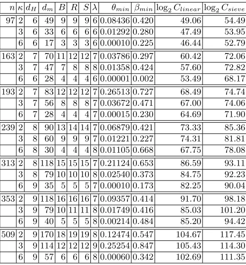
Table 3.Suitable values of parameter of improved FFS to solve DLP overGF(36n)
n κ dH dm B R S λ θmin βminlog2Clinear log2Csieve
97 2 6 49 9 9 9 6 0.08436 0.420 49.06 54.49 3 6 33 6 6 6 6 0.01292 0.280 47.49 53.95 6 6 17 3 3 3 6 0.00010 0.225 46.44 52.79 163 2 7 70 11 12 12 7 0.03786 0.297 60.42 72.06 3 7 47 7 8 8 8 0.01358 0.424 57.60 72.82 6 6 28 4 4 4 6 0.00001 0.002 53.49 68.17 193 2 7 83 12 12 12 7 0.26513 0.727 68.49 74.74 3 7 56 8 8 8 7 0.03672 0.471 67.00 74.06 6 7 28 4 4 4 7 0.00015 0.230 64.69 71.90 239 2 8 90 13 14 14 7 0.06879 0.421 73.33 85.36 3 8 60 9 9 9 7 0.01221 0.227 74.31 81.81 6 8 30 4 4 4 8 0.01105 0.668 67.75 78.08 313 2 8 118 15 15 15 7 0.21124 0.653 86.59 93.11 3 8 79 10 10 10 8 0.02540 0.373 84.75 92.23 6 9 35 5 5 5 7 0.00010 0.173 82.25 90.04 353 2 9 118 16 16 16 7 0.09357 0.414 91.70 98.18 3 9 79 10 11 11 8 0.01749 0.416 85.03 101.20 6 9 40 5 5 5 8 0.00214 0.484 85.20 94.42 509 2 9 170 18 19 19 8 0.12474 0.547 104.67 117.45 3 9 114 12 12 12 9 0.25254 0.847 105.43 114.30 6 9 57 6 6 6 8 0.00060 0.342 102.69 111.35
n: extension degree of the fieldGF(36n) over its base fieldGF(36)
κ: extension degree of the coefficient field ofGF(3κ)[x] such thatGF(36n)'GF(3κ)[x]/(f), wheref∈GF(3κ)[x] is a monic irreducible polynomial of degree 6n/κ
dH: degree inyof the bivariate polynomialH(x, y) =x+ydH ∈GF(3κ)[x, y] used for FFS dm: degree of the polynomialminGF(3κ)[x] such thatH(x, m)≡0 (modf)
B: smoothness bound for FFS
R: maximum degree of polynomialr∈GF(3κ)[x] used in the sieving step of FFS S: maximum degree of polynomials∈GF(3κ)[x] used in the sieving step of FFS λ: threshold value for the large prime variation
θmin: minimal ratio of the required special-Q’s to all monic irreducible polynomials inGF(3κ)[x] of degreeB
βmin: minimal ratio of the required large primes to all monic irreducible polynomials inGF(3κ)[x] of degreeB
Therefore, we suppose that the same property holds forn >97. Since the computational costs of (22) are very heavy when κ= 1 andn≥163, we omit the test for the condition.
Finally, for each fixed value of (n, κ, dH, dm, B, R, S, λ) mentioned above, we have computedβmin, θmin,
and obtained the costsCsieve, Clinear. Comparing these costs where (n, κ) is fixed and (dH, dm, B, R, S, λ)
is changed, we obtain Table 5 of suitable values of (dH, dm, B, R, S, λ, θ, β) for each fixed (n, κ).
Notice that in Table 5,Csieve for a fixed (n, κ) is larger thanClinear for the same (n, κ). Moreover,
for eachn, theCsieve withκ= 6 is less than theCsievewithκ= 2,3. Therefore, we estimate that the
time complexity of solving our DLP by the improved FFS isCsieve withκ = 6, so we obtain Table 1
and Figure 1. For each pair (n, κ, dH, dm) in Table 5, we have confirmed the existence of polynomials f, m, H satisfying (1), and these are given in Appendix D.
50 60 70 80 90 100 110 120 130
97 163 193 239 313 353 509
Complexity (log
2
)
degree n
L36n[1/3,(32/9)1/3] Our estimation
Fig. 1.Time complexity estimation of solving DLP overGF(36n) andL36n[1/3,(32/9)1/3] witho(1) =−0.18
6 Conclusions
In this paper, we evaluated the security of pairing-based cryptosystems using the ηT pairing defined
over finite fields whose characteristic is 3. For the evaluation, we consider the time complexity of solving the discrete logarithm problem (DLP) over the extension field GF(36n) of the embedding degree 6 by the asymptotically fastest function field sieve (FFS). The extension degree 6 allows us to improve the speed of FFS by efficient algorithms such as the large prime variation, lattice sieve, filtering, Galois action, and free relation. We therefore estimated the precise time complexity of solving our DLP by FFS with the efficient algorithms, called the “improved FFS” in this paper. By using our new formulas to count the explicit number of smooth polynomials used in the improved FFS, our experiment obtain the precise time complexity. Finally, we adapted the formulas to the degree n
Many high-speed implementations of the ηT pairing have been reported, which have attracted us
to achieve practical use of theηT pairing. Our estimation in this paper contributes to evaluating the
key length of the pairing-based cryptosystems using theηT pairing.
References
1. L. M. Adleman, “The function field sieve,” ANTS-I, LNCS 877, pp. 108-121, (1994).
2. K. Aoki, T. Shimoyama, and H. Ueda, “Experiments on the linear algebra step in the number field sieve,” IWSEC 2007, LNCS 4752, pp. 58-73, (2007).
3. L. M. Adleman and M.-D. A. Huang, “Function field sieve method for discrete logarithms over finite fields,” Inform. and Comput., vol.151, pp. 5-16, (1999).
4. O. Ahmadi, D. Hankerson, and A. Menezes, “Software implementation of arithmetic inF3m,” WAIFI 2007, LNCS 4547, pp. 85-102, (2007).
5. E. Barker, W. Barker, W. Burr, W. Polk, and M. Smid, “Recommendation for key management - Part 1: General (Revised),” NIST Special Publication 800-57, (2007).
6. P. S. L. M. Barreto, H. Y. Kim, B. Lynn, and M. Scott, “Efficient algorithms for pairing based cryptosystems,” CRYPTO 2002, LNCS 2442, pp. 354-368, (2002).
7. P. S. L. M. Barreto, S. Galbraith, C. ´O h ´Eigeartaigh, and M. Scott, “Efficient pairing computation on supersingular abelian varieties,” Des., Codes Cryptogr., vol.42, no.3, pp. 239-271, (2007).
8. J.-L. Beuchat, N. Brisebarre, J. Detrey, E. Okamoto, M. Shirase, and T. Takagi, “Algorithms and arithmetic operators for computing theηT pairing in characteristic three,” IEEE Trans. Comput., vol.57, no.11, pp. 1454-1468, (2008). 9. D. Boneh and M. Franklin, “Identity based encryption from the Weil pairing,” SIAM J. Comput., vol.32, no.3, pp.
586-615, (2003).
10. S. Cavallar, “Strategies in filtering in the number field sieve,” ANTS-IV, LNCS 1838, pp. 209-231, (2000).
11. S. Galbraith, K. Harrison, and D. Soldera, “Implementing the Tate pairing,” ANTS 2002, LNCS 2369, pp. 324-337, (2002).
12. E. Gorla, C. Puttmann, and J. Shokrollahi, “Explicit formulas for efficient multiplication inF36m,” SAC 2007, LNCS 4876, pp. 173-183, (2007).
13. R. Granger, “Estimates for discrete logarithm computations in finite fields of small characteristic,” Cryptography and Coding. LNCS 2898, pp. 190-206, (2003).
14. R. Granger, A. J. Holt, D. Page, N. P. Smart, and F. Vercauteren, “Function field sieve in characteristic three,” ANTS-VI, LNCS 3076, pp. 223-234, (2004).
15. R. Granger, D. Page, and M. Stam, “Hardware and software normal basis arithmetic for pairing-based cryptography in characteristic three,” IEEE Trans. Comput., vol.54, no.7, pp. 852-860, (2005).
16. D. Hankerson, A. Menezes, and M. Scott, “Software implementation of pairings,” In Identity-Based Cryptography, pp. 188-206, (2009).
17. K. Harrison, D. Page, and N. P. Smart, “Software implementation of finite fields of characteristic three, for use in pairing-based cryptosystems,” LMS Journal of Computation and Mathematics 5, pp. 181-193, (2002).
18. T. Hayashi, N. Shinohara, L. Wang, S. Matsuo, M. Shirase, and T. Takagi, “Solving a 676-bit discrete logarithm problem inGF(36n),” PKC 2010, LNCS 6056, pp. 351-367, (2010).
19. A. Joux et al, “Discrete logarithms inGF(2607) and GF(2613),” Posting to the Number Theory List, available at
http://listserv.nodak.edu/cgi-bin/wa.exe?A2=ind0509&L=nmbrthry&T=0&P=3690, (2005)
20. A. Joux and R. Lercier, “The function field sieve is quite special,” ANTS-V, LNCS 2369, pp. 431-445, (2002). 21. A. Joux and R. Lercier, “The function field sieve in the medium prime case,” EUROCRYPT 2006, LNCS 4004, pp.
254-270, (2006).
22. Y. Kawahara, K. Aoki, and T. Takagi, “Faster implementation ofηT pairing overGF(3m) using minimum number of logical instructions forGF(3)-addition,” Pairing 2008, LNCS 5209, pp. 282-296, (2008).
23. T. Kleinjung, K. Aoki, J. Franke, A. K. Lenstra, E. Thom`e, J. W. Bos, P. Gaudry, A. Kruppa, P. L. Montgomery, D. A. Osvik, H. J. J. T. Riele, A. Timofeev, and P. Zimmermann, “Factorization of a 768-Bit RSA Modulus,” CRYPTO 2010, LNCS6223, pp. 333-350, (2010).
24. T. Kerins, W. Marnane, E. Popovici, and P. S. L. M. Barreto, “Efficient hardware for the Tate pairing calculation in characteristic three,” CHES 2005, LNCS 3659, pp. 412-426, (2005).
25. C. Lanczos, ”Solution of systems of linear equations by minimized iterations,” J. Res. Nat. Bureau of Standards, vol.49, no.1, pp. 33-53, (1952).
26. A. K. Lenstra, H. W. Lenstra, Jr., M. S. Manasse, and J. M. Pollard, “The number field sieve,” LNIM 1554, pp. 43-49, (1993).
27. J. M. Pollard, “The lattice sieve,” LNIM 1554, pp. 43-49, (1993).
29. C. Pomerance and S.S. Wagstaff, Jr., “Implementation of the continued fraction integer factoring algorithm,” Congress. Numer., vol. 37, pp. 99-118, (1983).
30. N. Smart, D. Page, and F. Vercauteren, “A comparison of MNT curves and supersingular curves,” Applicable Algebra in Engineering, Communication and Computing, vol. 17, pp. 379-392, (2006).
A Function ¯ai,j used in Granger’s formulas and our new formulas
This appendix gives the formula of ¯ai, j used in the formula (15) in section 3.2 and in Theorem 1 in
section 4.3. In the same manner as Granger’s method [13], ¯ai, j is described as
¯
ai,j =
(q−1)2qi+j−1(i, j >0) (q−1)2qi (i= 0) (q−1)2qj (j= 0).
(23)
This corresponds to the equation (3) in [13]. Note that we suppose that 0≤i≤j in [13], but 0≤i, j
in this paper.
B Proof of formulas used in Theorem 1
This appendix gives proofs of formulas ρ2 and ρ3 used in Theorem 1 in section 4.3. Formulas ρ2 and ρ3 contain the formula Nq(k, B) that means the number of monic polynomials g of degree k, such
thatg is factorized into irreducible polynomials whose degree is not larger thanB. The details of the formulaNq(k, B) are given in [13].
B.1 Proof of formulas ρ2
ρ2(q, B, β, λ, k) =
1
qk
Nq(k, B−1) +
bk/B∑c
`≥1
Nq(k−`B, B−1)
min∑{`,λ}
i=1
(
bβIq(B)c i
)(
`−1
`−i
)
Proof .Letg∈GF(q)[x] be a monic irreducible polynomial of degreek and (B, β, λ)-smooth.
First we consider that the case g does not have any large primes, namely g is (B−1)-smooth. Then the number of such polynomials of degreek isNq(k, B−1).
Next we suppose that g has at least one large prime. Let sbe a (B−1)-smooth polynomial, and
tj a large prime factor ofs. Then g is described as follows:
g=s i
∏
j=1 tej
j (1≤i≤λ, ej ≥1).
Since the degree of polynomialsisk−`B where`=∑j=1i ej, there existNq(k−`B, B−1) candidates
ofsfor givenB and`. Here we consider the number of candidates of∏ij=1tj(x)ej. We selectidistinct
large primest1, ..., tifrom the setΛwhose cardinality isbβIq(B)c. Additionally, we select`−irepeated
polynomials from the set{t1, ..., ti}. Therefore, the number of candidates of
∏i
j=1tj(x)ej is
(
bβIq(B)c i
)(
i+ (`−i)−1
`−i
) =
(
bβIq(B)c i
)(
`−1
`−i
)
Consequently, since 1≤i≤λand 1≤`≤ bk/Bc, the number of candidates ofg is
bk/B∑c
`≥1
Nq(k−`B, B−1)
min∑{`,λ}
i=1
(
bβIq(B)c i
)(
`−1
`−i
)
There are qk monic polynomials of degree k, so we obtain that
ρ2(q, B β, λ, k) =
1
qk
Nq(k, B−1) +
bk/B∑c
`≥1
Nq(k−`B, B−1)
min∑{`,λ}
i=1
(
bβIq(B)c i
)(
`−1
`−i
)
B.2 The proof of formulas ρ3
ρ3(q, B, β, λ, Θ, k) =
1
qk
bk/B∑c
`=1
Nq(k−`B, B−1)
`
∑
`Q=1
min{`∑Q,λ,#Θ}
λQ=1 (
#Θ λQ
)(
`Q−1 `Q−λQ
)
τB,β,λ,Θ(`, `Q, λQ)
where
τB,β,λ,Θ(`, `Q, λQ) =
∑M in λt=1
(bβIq(B)c−#Θ
λt
)(`−`Q−1
`−`Q−λt )
(M in≥1)
1 (`=`Q),
0 (others),
M in= min{`−`Q, λ−λQ,bβIq(B)c −#Θ}.
Proof. Let Θ0 be the set Λ\Θ. Let g be a monic and (B, β, λ, Θ)-smooth polynomial in GF(q)[x] of
degree k.
First we suppose thatg has at least one prime factor in Θ0, sog is described as
g=s
(λ t ∏
i=1 tei
i ) λQ ∏ j=1 Qej
j
(ti∈Θ0, Qj ∈Θ), (24)
whereλt, ei, λQ, ej ≥1 andsis a (B−1)-smooth polynomial. Let `t, `Q be
∑λt
i=1ei,
∑λQ
j=1ej,
respec-tively. Then, there areNq(k−B(`t+`Q), B−1) such polynomialsssince degs=k−B(`t+`Q). Here
we consider the number of such∏λQ
j=1Qj(x)ej. We first selectλQdistinct polynomialsQ1, ..., QλQfrom
Θ, and then`Q−λQpolynomials are additionally selected from the set{Q1, ..., QλQ}. In this way, the product∏λQ
j=1Qj(x)ej are constructed, so the number of such product is
( #Θ
λQ
)(
λQ+ (`Q−λQ)−1 `Q−λQ
) = ( #Θ λQ )(
`Q−1 `Q−λQ
)
. (25)
In a similar way, the number of such∏λt
i=1ti(x)ei is
(
bβIq(B)c −#Θ λt
)(
`t−1 `t−λt
)
The number of such g is described as
bk/B∑c
`=2
Nq(k−`B, B−1)
`−1
∑
`Q=1
min{`Q∑,λ−1,#Θ}
λQ=1 (
#Θ λQ
)(
`Q−1 `Q−λQ
)
τB,β,λ,Θ(`, `Q, λQ)
,
(26)
where
τB,β,λ,Θ(`, `Q, λQ) = M in∑
λt=1 (
bβIq(B)c −#Θ λt
)(
`−`Q−1 `−`Q−λt
)
M in= min{`−`Q, λ−λQ,bβIq(B)c −#Θ}.
Since g is a (B, β, λ, Θ)-smooth polynomial, at most λ distinct polynomials can be selected from
Λ=Θ∪Θ0 for the product(∏λt
i=1t ei
i
) (∏λQ
j=1Q ej
j
)
. Thus we have that 2≤λQ+λt≤λ, so 1≤λQ≤
min{`Q, λ−1,#Θ}. By letting`=`Q+`t, we obtain that 2≤`≤ bk/Bc and 1≤`Q ≤`−1. Here
we consider the product(∏λt
i=1t ei
i
)
. Notice that`t=`−`Q, and in a similar way as above, we obtain
the properties for 1≤λt≤M in.
Then, we consider the case that ghas no factor in Θ0: namely g is factorized as
g=s
λQ ∏
j=1 Qej
j
(Qj ∈Θ). (27)
By extending (24) to the case thatλt=`t= 0, we can obtain the number of suchg. Notice that`=`Q
and 1≤λQ≤λ. There areNq(k−B`, B−1) such polynomialss, and the number of
∏λQ
j=1Qj(x)ej is
(25). Thus, the number of suchg is
bk/B∑c
`=1
Nq(k−`B, B−1)
min{∑`,λ,#Θ}
λQ=1 (
#Θ λQ
)(
`−1
`−λQ
)
. (28)
(28) is translated into
bk/B∑c
`=1
Nq(k−`B, B−1)
`
∑
`Q=`
min{`∑Q,λ,#Θ}
λQ=1 (
#Θ λQ
)(
`Q−1 `Q−λQ
)
. (29)
By adding (26) to (29), we want to describe the number of gas
bk/B∑c
`=1
Nq(k−`B, B−1)
`
∑
`Q=1
min{`∑Q,λ,#Θ}
λQ=1 (
#Θ λQ
)(
`Q−1 `Q−λQ
)
τB,β,λ,Θ(`, `Q, λQ)
Therefore, we define thatτB,β,λ,Θ(`, `Q, λQ) = 1 when`=`Q. The terms when`Q< `andλQ=λare
in excess, and we haveM in= 0 and`6=`Qunder the property. Hence, by extendingτB,β,λ,Θ(`, `Q, λQ)
to
τB,β,λ,Θ(`, `Q, λQ) =
∑M in λt=1
(bβIq(B)c−#Θ
λt
)(`−`Q−1
`−`Q−λt )
(M in≥1)
1 (`=`Q)
0 (others)
,
C Free relation in section 4.1
This appendix explains the number Rf ree (in section 4.1) of free relations. It is known that there
exist about # ˆF(B) free relations roughly [18]. However, if dH is divisible by 3, we obtain more free
relations.
Leta, bbe nonnegative integers such thatdH = 3aband gcd(3, b) = 1. We suppose thatq= 3κand
p∈ F¯(B) of degree d. Then, for any ti ∈ GF(q)[x]/(p), there exists an element ti+1 ∈ GF(q)[x]/(p)
such thatti =t3i+1. Therefore, we obtain that
H(x, y) =y3ab+x=y3ab+t31 = (y3a−1b+t1)3 =· · ·= (yb+ta)a.
Thus, the number of free relations is # ˆF ifb= 1.
Next we consider the case b= 2. If there exist T1, T2 satisfying that
y2+ta≡(y−T1)(y−T2) (mod p), (30)
then we obtain one free relation. The property (30) holds if and only if −ta is quadratic residue in GF(q)[x]/(p). Notice that the cardinality of GF(qd)∗ is even. Since exactly half of the elements in
GF(qd)∗ are quadratic residue, the probability that a random element inGF(qd)∗ is quadratic residue is 1/2. However, the probability for the fixed element −ta is required. We check (30) for every p, so
we guess that −ta behaves as a random element. Thus there are about # ˆF(B)/2 free relations, and
this fact is confirmed experimentally.
D Polynomials f and m used for function field sieve in section 2.2
This appendix gives example polynomialsf and m described in section 2.2 for the extension degrees
n and κ appearing in Table 3. The polynomials are represented by hexadecimal numbers in which “3” is substituted for the univariate polynomials f and m over GF(3κ) whose all coefficients are in GF(3). For example, the number 0x11327af4 (which is equal to 288520948 in the decimal number) of the polynomial m ∈ GF(36)[x] at the row of n = 97, κ = 6 means the univariate polynomial 2x17+ 2x15+ 2x12+ 2x11+ 2x10+x8+x6+x5+ 1.
• n= 97, κ= 2, dH= 6, dm= 49 m: 0x39964dda99f4afdc4b5a
f: 0x3f31f11476f4d1f90974a848f7a230e0f58abf660c549f80140176fe8eb6cf4c60f72a4fa07b11f5b589953b5f9b8627b71fd169a4d 0c5937495
• n= 97, κ= 3, dH= 6, dm= 33 m: 0x2bb4276d9b04a6
f: 0x1631a97eb594a8efc51f327df6b0ce76fd036bf6b34e6b9309d1ec2f3f56410e7e301d77f68d70 • n= 97, κ= 6, dH= 6, dm= 17
m: 0x11327af4
f: 0x4d31960ccaf29169980134a47469d224a84f489 • n= 163, κ= 2, dH= 7, dm= 70
m: 0x8e3f3c5cb849b6a9f1baa5dc021c
f: 0x10594fc2d06a45c0980736ce3d3f8d111bde1a984e87690d6e91ec6cc9e4ad1aea205407ea29478c5d2bebc2734417994f267992465 a74837712662e2c1cdfe4b35a191147aa06eb37c2cbd054b5e2017f8055ae53c3b8d06f5b20a6ebd88057060
• n= 163, κ= 3, dH= 7, dm= 47 m: 0x9670f0eb1b14b846a60
f: 0x266f4241d517bbb4ed2e65c9e7dc9c4a0537a8a9c75297ac57f9a16784ce63ac591015d0937ea0b095ddc52b9bdebc58a7e78cc1b11 07bd54f4d3cd623761a0f67
• n= 163, κ= 6, dH= 7, dm= 24 m: 0x72e1099b86
f: 0x96b90dd695d79212e2ff1b2ea804a6f49a615cd53ff16674bbf271457d6f4056e • n= 193, κ= 2, dH= 7, dm= 83
f: 0x3ae84fba553a71c0d63f23ac129cef4b3908f5fc5332eb2e9d47f3a028ff4403632585d9e2d90d3725c00f2d8898a56db64f1489166 47df2e474aef89bdb1e24e2bfa6895471812a5474de67149b3048034fabbe08a4bdc4cde32db9d88458f369d3a5f2f5ab9e070bf0cddb 8577667f346bdd
• n= 193, κ= 3, dH= 7, dm= 56 m: 0x4345d8983748633fa31bdb4
f: 0x191dd6323aa7ac2e93aaec774dfe0c05a10e281f5954c0ab86afa23c5daf333aca704f131a634a26106398b65ad92dfa370780f3f00 0759ef2d60ea145101fe95a1a86d7c2383e5b00982b75e9
• n= 193, κ= 6, dH= 7, dm= 28 m: 0x1ef3e12ae074
f: 0x5d10818cea67e0a5bd896a111e6a29af1cd1a4fbaf3c65638c00679732179454dda79852def62 • n= 239, κ= 2, dH= 8, dm= 90
m: 0x120758d4f8d47aca740b362c5a6d7d7dce858
f: 0x184cfc7460bab501388fde6826845bbdef023294c436aa97190038b3a09f8df41572b0b9873cb988ed4acb1a287270c75b71a6e7ae0 9f9cdf841fb3e7dd1dcdff1fa41148b997cfe9bfa636226eae48e9e032da7b72815f25e1b2804ca8a1d49af17f6a9daf6a172ad01537a 0f0445720291ce565aea27dbdca8ffafaf8fa239be5f6a67867b99f8c7819b3914583
• n= 239, κ= 3, dH= 8, dm= 60 m: 0x18bd6e17a060c429b5078f40f
f: 0x3be4d85c45e866a2446f06d8a393f68596cc41cb491c29d8b06ce94c2f5165e8fda191c059eb1039b54f091f1311c49dd84f173d2cf c1280e4d138e46e5f22e2aff3bdb111a3222fdb812016925b3ba587cc52fc506eab4d826c0da116ed06
• n= 239, κ= 6, dH= 8, dm= 30 m: 0xc55d20ceaebd
f: 0x7c161894e37f675847384d657397d87bc1f27b3b673bea716d58cbd4ec61d9102fb575905bd5dd0c0f5386715adbd4e • n= 313, κ= 2, dH= 8, dm= 118
m: 0x15b85b97c176e38a10e628fce756e29066d2699d78940788
f: 0x24d68c68a19d0d7841ade22df4ede00dee0da9b3815e3866f7a6b9b00615c0d06b201a236d362cc1aa6a8badb1d92a376d060a14325 a8e1327f9c7c8774c6b2e49c7d0a469139560f7a232ce4ef2e709e855546deb74886e27978afbb56cce283ef73173c9331e1e40955c57 e3209d66b46cc58db526cad3ff26b57ddfdb9ca7327a8fdd8da43c093f7e6852986b14deb28125c9e134dd86bac944bc87c5fe0808d29 6f2ad352384bd22b8aa6556f7faf63ba4233c60721d6aca8
• n= 313, κ= 3, dH= 9, dm= 79 m: 0x5655d29bdb485085208fd978abd42def
f: 0x20eb9bb0e7e0b2f97bdc7a49e4ea4f72ed4faa1ac9fccab08ed1468b2e1c387274874b3a1a7fc07999f6f8f6a4d02d1c84a8673c9d0 470ebc92d368e6aea4ffbaef34bd175a0f1bfe809d6f0a169b885eba260a24ae9fe122308a6fcc9b9940f3fce20be814fbf9fa9793b9c eb21d67587325d84d6b7e5eeaea7a9a68
• n= 313, κ= 6, dH= 9, dm= 35 m: 0x12b946308a71c98
f: 0x20c25be993cf520cfe972d4aa5b9f8f6fabafb0ee95c12f4ee748090eff153a9615e8167c2cc652e4aa95be03a5bd77095cb412791e 82cb71f3ae019593d8
• n= 353, κ= 2, dH= 9, dm= 118
m: 0x16968ca44e6ebff0cd072d643f88d9eb89b922eef48e6378
f: 0xa23742483db4f40824d9b2a7dabe6ff07ec5f15aa0d02deb59d0ed4d685f69c0942e1690b6fa452445320dbb0577ef57d2721d71951 54c3dcf0699b298fdb81fd4924d7c89c9e2eec93d65e03c53cafe11320c47f8d8cf45ea0950c63889e523cdf10fb01f1385ed2e0d45df b9393269db19265374d129d8e7a9c5e5f67f78d2072a9a9a0aa98448c3d22bf29cdba283080fb9bff4ba8e2309a2de1174be45221f9a2 baf13bfc71dfc639d98c1521d523f829cbf0bdec5f74cebac4bd5e17c9b4de51d9d3522efbe4e579592a8b745b64144
• n= 353, κ= 3, dH= 9, dm= 79 m: 0x368258f92e30a5a9f4385ac2543ba51c
f: 0x926ef1ee517c3cc5abfa767e929f5a4ec894381704939bdc27eb267e5411f6de25ef587c755220205763be7331660f915182d8a291f f6c7fc1a5efcc45c4c1806d702ac1214510a293cb674df27ff775e413a651ca9043097c0a817c424869bbdfcb59d2f30c68084993ec0b 6b7813e2f962e1711c39370555080eb85a7a272e05ebefaf13292cd8b7731212
• n= 353, κ= 6, dH= 9, dm= 40 m: 0x1544ad320c2775609
f: 0x159f625b2865ae374f202a8edeb3c5e715434d553dcfb0c211aff94b7c88395766aaa2da8903274f099f8a34088ebc1ce5574e7eb2e eca724530eb0de477ca546c29304b01f51
• n= 509, κ= 2, dH= 9, dm= 170
m: 0x637b0ddbb456ce4ca9c52bb1eba3060e2c8a560cd54e78caa05c37dcc331dbd1b22d
f: 0x197830517df44aa2772514e71875163887a269479f0fcb261ed5240c8bddb77db6b7e4d48ecf2c3b91895b3fff9e77bd225082cfe5f 8edb1ab8ae20394fd824f883b28edd5c04dfac56e7f4a00402d37c1bc40395787e126d5906d91705e1dcd7848f4caccd4c96c63eab14e 27671c1f47239f2cac87394971083610ecc082f9d7e2011a0f8ff09dc01ed94e201ad89efd0ca6e3c410a1d6940cdc5faf8287d35178b 5d94d1ea3b2b0fb4afc90e0c91ecaafd4133a4420616b1bcb35b8632a4b8d6f6efa9a8160e1b9f1927da7d91a90338e72ea11643faabc 0762d8d36ef3b4bb5ff8364a2284e88eb1cfcd0de4af34741618accf9c5a2c2d9b9abb7d1364d69d77d6a7d2b0558942c34fb38bc9856 dc5947a0f9a8b5e36b070d6975585b6b5b8977540b00f106be205c7407c040d
• n= 509, κ= 3, dH= 9, dm= 114
m: 0x1f34758909ee31a9e4666c6ab3d268a272e6abffd434f6
f: 0x5225d1ea2d9c5173cd7956accba48d7d0c00b321883dab86178ea0291ffc16c86cb68753e1b743d1117ad2a328a5565eb6b8ba4c141 fe67bc3380d842d8f2703ac8e7d3afddbaf66e88bc753bce09c47236f3907526d3bef3be36910ed61e723143c81dc14142c9b190a311a 1ca0835353de681ec18c301ee6394ccd702b1f2b904363e8e82176327a6e563410104d707ade6c1f58a98aced56103f113b814498d56c 755ca0da8ab1b5be29c6db7ef6624beb0bf545efe0b222c6a455369d4c56b7fcf1bbff942d8a144
• n= 509, κ= 6, dH= 9, dm= 57 m: 0x759368a35ffb3865a07a4aa
![Fig. 1. Time complexity estimation of solving DLP over GF(36n) and L36n[1/3, (32/9)1/3] with o(1) = −0.18](https://thumb-us.123doks.com/thumbv2/123dok_us/7894638.1310307/12.595.147.449.238.453/fig-time-complexity-estimation-solving-dlp-gf-l.webp)
