40
A Multi-objective continuous covering location model
Seyed Javad Hosseininezhad1*,mohammad Saeed Jabalameli2 1Industrial Engineering Department, K. N. Toosi University of Technology, Tehran, Iran
2
Industrial Engineering Department, Iran University of Science and Technology, Tehran, Iran
Abstract
This paper presents a multi-objective continuous covering location problem in fuzzy environment. Because the covering radius is assumed to be uncertain, this paper uses the possibility concept. Since uncertainty may cause risk of uncovering customers, the problem is formulated as a risk management model. The presented model is an extension of the discrete covering location model to continuous space. Two variables, namely selecting zone variable and covering variable are introduced for extending the discrete model to the continuous one. In the model, a facility is located in a zone with a predetermined radius from its center and is determined by the selecting zone variable. Allocating a customer to a facility is shown by a covering variable. Also, the paper introduces the possibility of covering, based on distance between the customers and the facilities. Two objectives are considered in the model; the first is the possibility of covering by each facility and the second is the risk cost of the uncovered customers. Fuzzy programming is applied for converting the model to a single objective one. Finally, a numerical example with sensitivity analysis is expressed to illustrate the presented model.
Keywords: continuous covering location problem (CCLP); risk management; fuzzy covering radius; multi objective problem.
1- Introduction
The covering problem aims to locate a set of new facilities in a manner that the customers can receive service by each facility that its distance to customer is equal or less than a predefined value. This critical value is called coverage. Church and ReVelle (1974) are the one of the first researchers that modeled the maximization covering problem. The covering problem is divided into two problems; the total covering and the partial covering based on covering all or some of the demand points. The total covering problem is modeled by Toregas (1971). Up to the present time many developments have been occurred about the total covering and the partial covering problems in solution techniques and assumptions. The covering problem has many applications such as: the design of switching circuits, data retrieving, assembly line balancing, airline staff scheduling, locating defend networks, distributing products, warehouse locating and location of emergency service facility (Francis et al. 1992).Some researchers such as Church and ReVelle (1974), Schilling et al. (1993), Owen and Daskin (1998) and Drezner and Wesolowsky (1999) investigated network covering problems.
The total covering problem cannot cover all location problems in real world, because in many problems budget constraint and other constraints do not let us cover all the points and there is a risk of having unsatisfied customers. In this paper the partial covering model is investigated.
*Corresponding author.
ISSN: 1735-8272, Copyright c 2016 JISE. All rights reserved Journal of Industrial and Systems Engineering
Vol. 9, special issue on location allocation and hub modeling, pp 40-52 Winter (February) 2016
41
Mirchandani and Francis (1990) provided a covering model in discrete space. Assuming that there are n demand points indexed by I, and k candidate locating points indexed by j and Pi is the penalty of not covering demand point i, the model is written as the following.
) 1 (
:
st:
) 2 (
+ ≥ 1, ∀ = 1,2, … ,
∈ 0,1 , ∈ 0,1 , ∀ = 1,2, … , ∀ = 1,2, … ,
Where,
: is 1 if the candidate locating point j can cover the demand point i , otherwise is 0
( ’s constitute the covering matrix)
: is 1 if a facility is located at the candidate locating point j, otherwise is 0 : is 1 if the demand point i is not satisfied, otherwise is 0
Equation (1) is the objective function consisting of the penalty costs. Constraint set (2) guarantees that is 1 if is zero, it means that the demand point i is not covered. The above model and other related covering location models have been investigated only in discrete space; while there are situations that might occur in continuous space. In this paper, we introduce a continuous covering location problem and for more adopting on real world, we consider the model in uncertain conditions by considering the fuzzy covering radius and providing the final problem as a risk management model. We are interested in finding location of k facilities in continuous space in order to serve the customers at n demand points so that the total cost of uncovered customers is minimized and the possibility of coverage by each facility is maximized.
Basic information underlying a facility location problem includes demand levels, travel time or cost for supplying the customers, location of the customers, presenceor absence of the customers, and price for the commodities. Uncertainty may occur in one or several of these parameters. In this condition, we make a decision under risk and we can apply methods for dealing with the problem (Laporte et al., 2015). Investigating risk is one of the main topics in location models. The main factors which lead to risk could be categorized as uncertain parameters such as production, demand, supplies, processing, transportation, inventory, capacity, cost, interest rate and etc. Robust optimization, stochastic programming, chance-constrained models and fuzzy approaches are applied for considering uncertainty in location models.
The reminder of the paper is organized as follows; in section 2 a literature review about the covering location model in fuzzy environmentand risk management in the location models are provided. In section 3 we present Continuous Covering Location Problem (CCLP). The final multiobjective model and fuzzy programming for converting the multiobjective model to the single objective one is provided in section 4. In section 5 and section 6 a numerical example with sensitivity analysis is given to illustrate the usability of the presented model. Finally, Section 7 draws the conclusions and future works.
2
- Literature Review
Several researchers have investigated the covering location model in fuzzy environment. Li et al. (2002) considered two fuzzy versions of the well-known problem of determining the smallest circle that would cover a given finite set of points in the plane when the locations of points are not precise but fuzzy. The first was modeled as a possibility-constrained mathematical program and the second, as a necessity-constrained one. Berman et al. (2003) considered the concept of a gradual coverage by introducing two distances on a network. A demand point is fully covered if it is within the lower distance, not covered at all if it is beyond the larger distance, and, if its distance is between the two distances, a level of coverage is determined using a decay function. Perez et al. (2004) claimed that in real applications facility locations can be full of linguistic vagueness that can be appropriately modeled using networks with the fuzzy values which describe nodes. Chiang et al. (2005) developed the fuzzy set-covering model using auxiliary 0-1. Chiang et al. (2005) proposed a set-set-covering model using the concept of fuzzy set theory to define fuzzy covers. Huang et al. (2006) analyzed a linear feature covering problem with distance constraints, and characterized the problem by a fuzzy multi objective optimization model. Shavandi and Mahlooji (2006) utilized fuzzy theory to develop a queuing maximal covering location–allocation. Araz et al. (2007) considered a multi-objective maximal covering location model. The model addresses the issue of determining the best base locations for a limited number of vehicles so that the service level objectives are optimized. The
42
objectives of the model are maximization of the population covered by one vehicle, maximization of the population with backup coverage and minimization of the total travel distance in locations more distant than a prespecified distance standard for all zones. Ni (2008) considered the edge covering problem under fuzzy environment, and formulated three models which are expected minimum weight edge cover model, α-minimum
weight edge cover model, and the most minimum weight edge cover model. Batanovic et al. (2009) investigated a class of maximum covering location problems in networks in uncertain environments. They assumed that relative weights of demand nodes are either deterministic or imprecise. Sirbiladze et al.(2009)introduced a new criterion for minimal fuzzy covering problems, which is the minimal value of the average misbelieve contained in the possible alternatives.
Several researches have been concentrated on considering risk in facility location problem. Guillen et al. (2005) considered the design and retrofit problem of a supply chain consisting of several production plants, warehouses, markets and the associated distribution systems. They constructed a two-stage stochastic model in order to take the effects of the uncertainty in the production scenariointo account. Snyder et al. (2007) proposed a stochastic version of the location model with risk pooling which optimizes location, inventory and allocation decisions under random parameters described by discrete scenarios. The goal of their model was to find solutions to minimize the expected total cost of the system among all scenarios. They presented a Lagrangian relaxation based exact algorithm for the model. Ozsen et al. (2008) introduced the capacitated warehouse location model with risk pooling. The model provided a logistics system in which a single plant shipped one type of product to a set of retailers, each with an uncertain demand. Also, the model was solved by a Lagrangian relaxation solution algorithm. Azaron et al. (2008) developed a multi-objective stochastic programming approach for supply chain design under uncertainty. Demands, supplies, processing, transportation, shortage and capacity expansion costs were all considered as uncertain parameters. They used the goal attainment technique to obtain the Pareto-optimal solutions. Afterwards, Wagner et al. (2009) considered a location-optimization problem where the classical incapacitated facility location model was recast in a stochastic environment with several risk factors that made demand at each customer site probabilistic and correlated with demands at the other customer sites. They considered “Value-at-Risk” (VaR) measure and designed a branch-and-bound algorithm to solve the problem. You
et al. (2009) proposed a two-stage stochastic linear programming approach within a multi-period planning model.
Furthermore, they developed an algorithm based on the multi-cut L-shaped method in order to solve the resulting large scale industrial size problems. Mete and Zabinsky (2010) developed a stochastic optimization approach for the problem of storage and distribution of medical supplies to be used for disaster management under a wide variety of possible disaster types and magnitudes. Cui et al. (2010) investigated reliable facility location models considering unexpected failures with site dependent probabilities, as well as possible customer reassignment. They proposed a compact mixed integer program formulation which was solved using a custom-designed Lagrangian relaxation algorithm. Liu et al. (2010) presented a location model that assigns online demands to the capacitated regional warehouses currently serving in-store demands in a multi-channel supply chain. The model explicitly considered the trade-off between the risk pooling effect and the transportation cost in a two-echelon inventory/logistics system. They formulated the assignment problem as a non-linear integer programming model. A strategic supply chain management problem was studied by Peng et al. (2011) to design reliable networks that perform as well as possible under normal conditions, while also performing relatively well when disruptions strike. They presented a mixed-integer programming model whose objective was to minimize the nominal cost while reducing the disruption risk using the p-robustness criterion which bounds the cost in disruption scenarios. Chen et al. (2011) presented a multi-criteria decision analysis for environmental risk assessment with regard to avoiding and eliminating damages and loss under natural disasters in international airport projects. They used the ANP to demonstrate one of its utility modes in decision making support to location selection problems, which aims to an evaluation of different projects from different locations.
A facility location model with fuzzy random parameters and its swarm intelligence approach was studied by Wang and Watada (2012). A VaR based fuzzy random facility location model was built in which both the costs and demands were assumed to be fuzzy random variables. The model was inherently a two-stage mixed 0–1 integer fuzzy random programming problem. A hybrid modified particle swarm optimization approach was proposed to solve the model. A corresponding framework for value-based performance and risk optimization in a single-stage supply chain problem was developed by Hahn and Kuhn (2012). They applied Economic Value Added as a prevalent metric of value-based performance to mid-term sales and operations planning. Due to the uncertainty of future events in a scenario based problem, they also used robust optimization methods to deal with operational risks in physical and financial supply chain management. Nickel S. et al (2012) provided a multi-period supply chain network design problem. In this problem, uncertainty was assumed for demand and interest rates, which was described by a set of scenarios. Accordingly, the problem was formulated as a multi-stage stochastic mixed-integer linear programming problem. Recently, Hosseininezhad et al. (2013) proposed a
43
continuous covering location model with risk consideration in which the objective function consists of installation and risk costs and introduced a risk analysis method based on Response Surface Methodology (RSM) to consider risk management in the location models. Also, Hosseininezhad et al. (2014) presented a continuous capacitated location-allocation model with fixed cost as a risk management model. In the presented model, the fixed cost consists of production andinstallation costs. The model considered risk as percent of unsatisfied demands.
In the rest of this section, aforementioned articles are classified based on location model, risk type, space and uncertainty as shown in Table 1 in order to help the reader appreciate the symmetry associated with the facility location problems.
In the next section, the continuous covering location model with risk consideration is introduced. Because of uncertain covering radius, the problem is formulated as a risk management model. Therefore, the main differences of our research compared to the mentioned works are as follows.
1. Providing a continuous model for the covering location problem
2. Investigating fuzzy coverage and possibility of covering in the covering location model. 3. Investigating risk in continuous space as a multiobjective model
3-
Continuous Covering Location problem (CCLP)
In this section, a continuous covering location model is introduced which is the extension of the model in continuous space. For this model, the space is divided into n zones.We are interested in finding the location of k facilities in continuous space. Assuming ! , " are the coordinates of the facility and , # are coordinates of the center of zone I (or the customer i ) and D is the maximum distance that a facility could be located from the center of a zone for assigning to the zone. Two new variables $ and % are also introduced in the model.$ , namely, the selected zone variable shows whether or not the facility j is located in the zone i; it is assumed that the distance between each customer and each facility is euclidean. Then constraints (3) and (4) are as follows.
) 3 (
$ &'(! − *++ (" −# *+, ≤ ., ∀ = 1,2, … ,
) 4 (
$ = 1, ∀ = 1,2, … ,
Table1. Comparison between the works
Uncertainty Space Risk type Location model Author(s) Stochastic Discrete Scenario based Multi objective supply chain
Guillen et al (2005)
Stochastic Discrete
Scenario Based Location with risk pooling
Snyder et al (2007)
Stochastic Discrete
Uncertain demand Warehouse location
Ozsen et al.(2008)
Stochastic Discrete
Scenario Based Multi-objective stochastic
Azaron et al.(2008)
Stochastic Discrete
Value-at-Risk Uncapacitated p-median
Wagner et al.(2009)
Stochastic Discrete
Uncertain demand Multi-product supply chain
You et al. (2009)
Stochastic Discrete
Disaster Location with vehicle routing
Mete and Zabinsky (2010)
Stochastic Discrete
Risk of disruption Reliable facility location
Cui et al.(2010)
Stochastic Discrete
Stochastic demand Two-echelon inventory/logistics
Liu et al. (2010)
Stochastic Discrete
Disruption Reliable logistics network design
Peng et al. (2011)
judgmental Discrete
Disaster Location selection
Chen et al. (2011)
Fuzzy Discrete
Value-at-Risk Fuzzy facility location
Wang and Watada (2012)
Stochastic Discrete
Scenario Based Single-stage supply chain
Hahn and Kuhn (2012)
Stochastic Discrete
Scenario Based Multi-stage supply chain
Nickel S. et al (2012)
Fuzzy Continuous
Uncertain covering radius Continues covering location
Hosseininezhad et al.(2013)
Fuzzy Continuous
Uncertain demand Continues location allocation
Hosseininezhad et al.(2014)
Fuzzy Continuous
Uncertain coverage Continues covering location
44
Constraint (3) guarantees that if the distance between the facility j and the zone i is greater than D,$ = 0, so the facility j won't be located in the zone i and the facility j will be located in the zone i, if the distance between the facility j and the zone i is smaller than D, constraint (4) Guarantees that the facility j is installed only in one zone. Also, we set a constraint to locate facilities in each zone as follows.
) 5 (
$ ≤ 1, ∀ = 1,2, … ,
Constraint (5) guarantees that at most one facility could be located in the zone i. Another new variable % , namely, the covering variableshows whether or not the customer i is covered by the facility j. If / is the covering radius and L is a large value, then
) 6 (
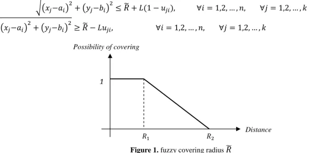
'(! − *++ (" −# *+ ≤ / + 0(1 − % ), ∀ = 1,2, … , , ∀ = 1,2, … ,
) 7 (
'(! − *++ (" −# *+ ≥ / − 0% , ∀ = 1,2, … , , ∀ = 1,2, … ,
Constraints (6) and (7) are the covering constraints and guarantee that each customer can be covered by a facility if the distance between them is smaller than/; % ’s (∀ = 1,2, … , ∀ = 1,2, … , ) constitute the covering matrix. If the distance between the customer i and the facility j is greater than / then % = 0 and % = 1 otherwise; since L is a large value constraint sets (6), (7) will be satisfied, simultaneously. Assuming that if the customer i is not covered by any of facilities, then 2 = 1,we set a constraint similar to constraint (2) as follows.
) 8 (
% + 2 ≥ 1, = 1,2, … ,
Constraint (8) indicates the demand constraint which guarantees that 2 is 1 if % is zero, it means that the customer i is not covered. If 3 is the importance of customer i, the objective function of the model constitutes of the risk cost which is the cost of the uncovered customers based on the importance of each customer. Accordingly, by integration (3)-(8), the continuous covering location model as the 0-1 nonlinear programming model +is as shown in (9):
) 9 (
+: 3 2
st:
$ &'(! − *++ (" −# *+, ≤ ., ∀ = 1,2, … ,
$ = 1, ∀ = 1,2, … ,
$ ≤ 1, ∀ = 1,2, … ,
'(! − *++ (" −# *+ ≤ / + 0(1 − % ), ∀ = 1,2, … , , ∀ = 1,2, … , '(! − *++ (" −# *+ ≥ / − 0% , ∀ = 1,2, … , , ∀ = 1,2, … ,
% + 2 ≥ 1, = 1,2, … ,
$ , % , 2 ∈ 0,1 ! , " ∈ ℝ∀ = 1,2, … , , ∀ = 1,2, … ,
45
4
- Multi objective continuous covering location model
In this section, at first the multiobjective model is presented and then a fuzzy programming is applied to convert the model to a single objective one. Since we investigate the problem in uncertain conditions, assuming the covering radius is a triangle fuzzy number/5 = (/ , / , /+) as shown in Figure1, in the model + we replace (6) and (7) by (10) and (11), respectively as follows.
) 10 (
'(! − *++ (" −# *+≤/6 + 0(1 − % ), ∀ = 1,2,…, , ∀ = 1,2,…,
) 11 (
'(! − *++ (" −# *+ ≥/6 − 0% , ∀ = 1,2,… , , ∀ = 1,2,…,
In this paper, we introduce the possibility of covering concept as follows. If the distance between a customer and a facility is smaller than / , the possibility of covering is 1, if the distance is greater than /+, the possibility of covering is 0 and if the distance is between / and /+, the possibility of covering is between 0 and 1.So,
) 12 (
7 =
8 99 : 99
;1 '(! − *++ (" −# *+≤ /
&/+−'(! − *++ (" −# *+, (/< +−/ ) / ≤ '(! − *++ (" −# *+≤ /+
0 /+≤ '(! − *++ (" −# *+
= ,∀ ,
According to constraint (12), 7 is the possibility of covering the customer i by the facility j and constraints (13) and (14) are provided as follows.
) 13 (
'(! − *++ (" −# *+− /++ 7 (/+− / ) ≤ 0(1 − % ), ∀ = 1,2, … , , ∀ = 1,2, … ,
) 14 (
7 ≤ 0% , ∀ = 1,2, … , , ∀ = 1,2, … ,
Constraints (13) and (14) are the possibility of covering constraints; since 0 ≤ 7 ≤ 1 and L is a large value, if the customer I can be covered by the facility j then % = 1 and the constraint (13) is activated. If % = 0 the constraint (14) is activated and 7 = 0. Constraints (13) and (14) guarantee feasibility of the model. Also for providing a crisp model, /5 is replaced by /+ which guarantees that if the distance between the customer i and the facility j is greater than /+,then % = 0.In the model +, the risk cost, namely>, is minimized. But because of uncertainty, it is desired to maximize the possibility of covering by facilities. So we add the possibility of covering concept by each facility, namely >+, to the model, then the multiobjective continuous location model ?is as provided in (15).
Figure 1. fuzzy covering radius /@
/ /+ Distance
1
46
) 15 ( ?:
8 9 : 9
;> : ! (3 ∙ 7 *B
>+: 3 2
C 9 D 9 E
S.t.
'(! − *++ (" −# *+≤ /++ 0(1 − % ), ∀ = 1,2, … , , ∀ = 1,2, … ,
'(! − *++ (" −# *+≥ /+− 0% , ∀ = 1,2, … , , ∀ = 1,2, … ,
% + 2 ≥ 1, = 1,2, … ,
$ &'(! − *++ (" −# *+, ≤ ., ∀ = 1,2, … ,
$ = 1, ∀ = 1,2, … ,
$ ≤ 1, ∀ = 1,2, … ,
'(! − *++ (" −# *+− /++ 7 (/+− / ) ≤ 0(1 − % ), ∀ = 1,2, … , , ∀ = 1,2, … ,
7 ≤ 0% , ∀ = 1,2, … , , ∀ = 1,2, … ,
$ , % , 2 ∈ 0,1 ,0 ≤ 7 ≤ 1, ! , " ∈ ℝ∀ = 1,2, … , , ∀ = 1,2, … ,
For converting the multiobjectivemodel ? to a single objective one a fuzzy programming is applied.At first, we solve two single models with the objective > and >+ , separately. If F and F+bethe obtained solution of > and
>+, respectively, we replace F and F+ in >+ and > , respectively, to obtain lower and upper bound for each objective, so a pay-off matrix is obtained as shown in Table 2.
Table 2. Pay-off matrix for the multi objective model
> (F) >+(F)
F > (F ) = G >+(F ) = G+
F+ > (F+) = 0 >
+(F+) = 0+
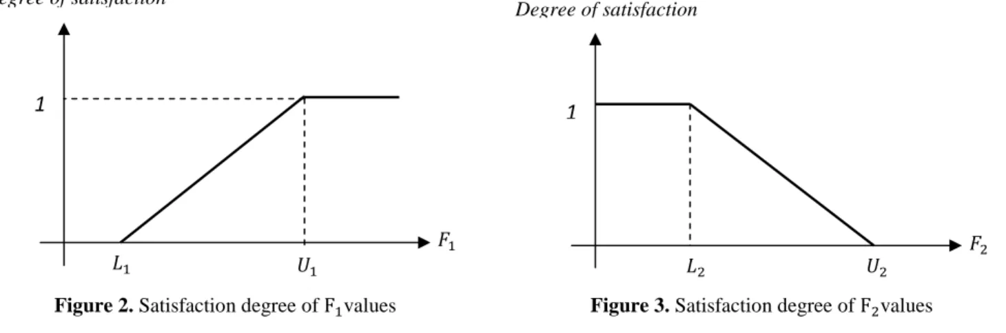
Two variables H (F) and H+(F) are introduced which are satisfaction degree of the objective values >and >+, respectively, then constraints (16) and (17) are as follows.
) 16 (
H (F) = 8 :
;0>1(F) −01 >1(F) ≤ 01 G1−01 01≤ >1(F) ≤ G1
1 G1 ≤ >1(F)
=
) 17 (
H+(F) =
8 :
;1G >2(F) ≤ 02
2− >2(F)
G2−02 02≤ >2(F) ≤ G2
0 G2 ≤ >2(F)
=
47
Figure 3. Satisfaction degree of F+values
Figure 2. Satisfaction degree of F values
Finally, we use Zimmermann Max-min operator as shown in constraint (18),
) 18 (
max min H (F), H+(F)
If O = min H F1, H+ F1 and 0 ≤ O ≤ 1, Since O ≤ H F1then, O ≤ > F1 − 0 1 G − 0 1⁄ , then constraint (19) is as follows,
) 19 (
0 − Q (3 ∙ 7 *B R + O G − 0 1 ≤ 0,
We carry out similar calculations for H+ F1which lead toconstraint set (20) as follows,
) 20 (
3 2 − G++ O G+− 0+1 ≤ 0
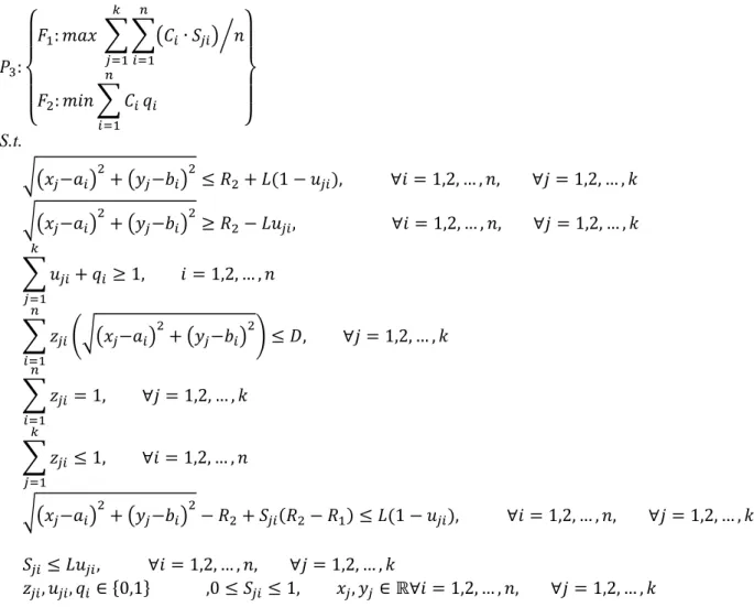
Then, the final single objective model Sis as provided in (21)
) 21 (
S: max O
st:
'(! − *++ (" −# *+≤ /++ 0 1 − % 1, ∀ = 1,2, … , , ∀ = 1,2, … ,
'(! − *++ (" −# *+≥ /+− 0% , ∀ = 1,2, … , , ∀ = 1,2, … ,
% + 2 ≥ 1, = 1,2, … ,
$ &'(! − *++ (" −# *+, ≤ ., ∀ = 1,2, … ,
$ = 1, ∀ = 1,2, … ,
$ ≤ 1, ∀ = 1,2, … ,
'(! − *++ (" −# *+− /++ 7 /+− / 1 ≤ 0 1 − % 1, ∀ = 1,2, … , , ∀ = 1,2, … ,
7 ≤ 0% , ∀ = 1,2, … , , ∀ = 1,2, … ,
0+
>+
G+
1
Degree of satisfaction
0 G >
1
48
0 − Q (3 ∙ 7 *B R + O G − 0 1 ≤ 0,
3 2 − G++ O(G+− 0+) ≤ 0,
$ , % , 2 ∈ 0,1 ,0 ≤ 7 ≤ 1, 0 ≤ O ≤ 1, ! , " ∈ ℝ∀ = 1,2, … , , ∀ = 1,2, … ,
Finally, O is the objective value, (! , " * provide the best location of the facility j and % ′U for i , j provide the covering matrix.
5-
Numerical example
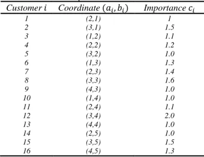
In this section, a numerical example is expressed to illustrate the introduced model. Suppose that we want to locate 3 new facilities in a region including 16 zones (customers). Specifications of customers are shown in Table 3. As shown in Figure4, Fuzzy covering radius is/5 = (0.70,0.70,1.10) andD=0.60.
Table 3. specifications of customers
Customer Coordinate ( , # ) Importance X
1 (2,1) 1
2 (3,1) 1.5
3 (1,2) 1.1
4 (2,2) 1.2
5 (3,2) 1.0
6 (1,3) 1.3
7 (2,3) 1.4
8 (3,3) 1.6
9 (4,3) 1.0
10 (1,4) 1.0
11 (2,4) 1.1
12 (3,4) 2.0
13 (4,4) 1.0
14 (2,5) 1.0
15 (3,5) 1.5
16 (4,5) 1.3
At first, we solve the model ? for the objective >and>+, separately, the example was solved by optimization software which uses the branch and reduce algorithm. The Pay-off matrix for the numerical example is as shown in Table 4.
Figure 4. fuzzy covering radiusR6 for the numerical example
0.70 1.10 Distance
1
49
Table 4. Pay-off matrix for the numerical example
> F1 >+ F1
F G = 0.273 G+ = 0.570
F+ 0 = 0.153 0
+= 0.165
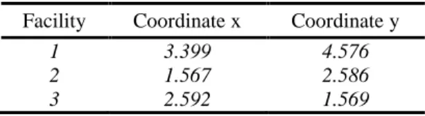
Finally, the model Sis solved and coordinates of new facilities are shown in Table 5. Table 5.Coordinate of new facilities
Facility Coordinate x Coordinate y
1 3.399 4.576
2 1.567 2.586
3 2.592 1.569
The covering variable and the selecting zone variables are
% , + = % , ?= % , ] = % , ^= %+,?= %+,S= %+,^= %+,_= %?, = %?,+ = %?,S= %?,]= 1.00
$ , ]= $+,_= $?,]= 1
As shown, the facilities are located in zones 5, 7 and 15. Also, the possibilities of covering values are
7 , += 1.00, 7 , ?= 0.67, 7 , ]= 1.00, 7 , ^= 0.91
7+,?= 0.71, 7+,S= 0.93, 7+,^= 1.00, 7+,_= 1.00
7?, = 0.70, 7?,+= 1.00, 7?,S= 0.92, 7?,]= 1.00 and,
2a= 2b= 2 c= 2 = 2 S= 1.00
That means customers 8,9,10,11,14 are not covered. Finally, the objective value isO = 0.702. The final solution is shown in Figure 5.
Location of customers Location of facilities
Figure 5. Results of the numerical example
6-
Sensitivity Analysis
In this section, we analyze the presented models based on the numerical example. At first, a sensitivity analysis is carried out for the CCLP model by changing parameter / which is shown in Figure6. As can be seen, by increasing the covering radius, the risk is decreased.This shows usability of the presented continuous covering location model +based on different covering radius.
50
Figure 6. Sensitivity analysis of the CCLP model
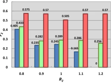
The final analysis deals with the importance of considering two objective functions simultaneously as introduced namely the multi objective continuous location model. Assuming > and >+ are the value of objective > in the model ? with merely the objective > and >+, respectively, and >+ and>++ are the value of objective >+ in the model ? with merely the objective> and >+, respectively, we solve the model ? by changing parameter /+with fixing / = 0.70, as shown in Figure 7 and Figure 8. Also, if >∗and >+∗are the values of the objective > and >+ obtained by solving the presented model with different /+ values, respectively. The best results for > are obtained via> but in this case the worst results for >+areobtained here. On the other hand, the best results for >+are obtained via >++but in this case the worst results for > are obtained here. Obviously considering merely one objective may sacrifice the other. Comparison of results shows that the presented model makes a tradeoff between these two objective functions.
Figure 7. Sensitivity analysis of the presented model
with merely the objectiveF
Figure 8. Sensitivity analysis of the presented model
with merely the objective F+
7-
Conclusion
This paper presents a multi objective continuous covering location problem in fuzzy environment as the risk management model. Because of uncertain covering radius, the possibility of covering concept was introduced. The presented model’s advantage over the traditional covering location ones was the consideration of continuous space for the covering problems. Two variables were introduced for extending the discrete model to the continuous one; the selected zone and the covering variables. Providing the continuous risk management location model is another usability of the presented model. Also, the paper introduces the possibility of covering based on the distance between the customers and the facilities. The two-objective modelwas constituted ofthe maximum possibility of
0 0.1 0.2 0.3 0.4 0.5 0.6
0.7 0.8 0.9 1 1.1 1.2
O b je ct iv e fu n ct io n R 0.218 0.244 0.264 0.273 0.285 0.203 0.228 0.249 0.237 0.231 0.13 0.127 0.175 0.153 0.165 0 0.05 0.1 0.15 0.2 0.25 0.3
0.8 0.9 1 1.1 1.2
F1
R2
F11 F1* F12
0.405 0.235 0.245 0.165 0 0.433 0.282 0.289 0.286 0.256 0.575 0.57 0.505 0.57 0.57 0 0.1 0.2 0.3 0.4 0.5 0.6 0.7
0.8 0.9 1 1.1 1.2
F2
R2
51
covering by each facility and the minimum risk cost of uncovered objectives. Then, the fuzzy programming was applied for converting the model to the single objective one. Finally, sensitivity analysis was carried out to show the usability's of the continuous covering location problem and the presented two-objective model. Extension of the model as a continuous covering location allocation model with uncertain supply and demand and considering uncertain budget could be investigated in future researches. Providing a heuristic method for large scale instances is another research issue which we think may need future investigations.
References
Araz C., Selim H., Ozkarahan I., (2007), “A fuzzy multi-objective covering-based vehicle location model for emergency services”, Computers & Operations Research, 34, 705–726.
Azaron A. et al., (2008), “A multi-objective stochastic programming approach for supply chain design considering risk”, International Journal of Production Economics, 116, 129-138.
Batanovic V., PetrovicD., PetrovicR.(2009), “Fuzzy logic based algorithms for maximum covering location problems”, Information Sciences, 179, 120–129.
Berman O., Krass D., Drezner Z., (2003), The gradual covering decay location problem on a network, European
Journal of Operational Research,151, 474–480.
Chen Z., Li H., Ren H., Xu Q., Hong J., (2011), “A total environmental risk assessment model for international hub airports”, International Journal of Project Management , 29, 856–866.
Chiang C. I. , Hwang M. J., Liu Y. H., (2004), “Solving a Fuzzy Set-Covering Problem”, Mathematical and
Computer Modelling, 40, 861-865.
Chiang C. I. , Hwang M. J., Liu Y. H., (2005), “An Alternative Formulation for Certain Fuzzy Set-Covering Problems”, Mathematical and Computer Modelling, 42 , 363-365.
Church R, ReVelle C., (1974), “the maximal covering location problem”, Papers Region. Sci. Assoc., 32,101–118. Cui T., Ouyang Y., Shen Z.-J. M., (2010), ”Reliable facility location design under the risk of disruption”,
Operation Research, 58, 998-1011.
De Boer P., Kroese D.P., Mannor S, Rubinstein R.Y., (2005), “A tutorial on the cross-entropy method”,Annals of
Operations Research, 2005,134(1):19–67.
Drezner Z., Wesolowsky G., (1999), “Allocation of discrete demand with changing costs”, Computers and
Operations Research, 26, 1335–1349.
Francis, R.L., F. Leon, L.F. McGinnis, and J.A. White, (1992), “Facility Layout and Location: An Analytical Approach” ,NY: Prentice Hall.
Guillen G., Mele F.D., Bagajewicz M. J., Espuna A., Puigjaner L., (2005), “Multiobjective supply chain design under uncertainty”, Chemical Enginnering Science, 60, 1535-1553.
Hahn G.J., Kuhn H., (2012), “Value-based performance and risk management in supply chains: A robust optimization approach”, International Journal of Production Economics, 139, 135-144.
Huang B., Liu N., Chandramouli M., (2006), “A GIS supported Ant algorithm for the linear feature covering problem with distance constraints”, Decision Support Systems, 42, 1063–1075.
Hosseininezhad S. J.,Jabalameli M. S.,JalaliNaini S. G, (2013), “A continuous covering location model with risk consideration”, Applied Mathematical Modelling, 37, 9665-9676.
Hosseininezhad S. J.,JabalameliM. S.,JalaliNaini S. G, (2014), “A fuzzy algorithm for continuous capacitated location allocationmodel with risk consideration”, Applied Mathematical Modelling, 38, 983–1000.
52
Huang B., Liu N., Chandramouli M., (2006), “A GIS supported Ant algorithm for the linear feature covering problem with distance constraints”, Decision Support Systems, 42, 1063–1075.
Laporte G., Nickel N., Saldanha da Gama F.,Editors, (2015), Location Science, Springer, Switzerland.
Liu K., Zhou Y., Zhang, Z. (2010), “Capacitated location model with online demand pooling in a multi-channel, supply chain”, European Journal of Operational Research, 207, 218–231.
Lushu L., Kabadi S. N., Nair K.P.K. (2002), “Fuzzy versions of the covering circle problem”, European Journal of
Operational Research, 137, 93-109.
Mirchandani P.B., Francis R.L., (1990), Discrete location theory. Wiley, New York.
Mete H. O., Zabinsky Z. B., (2010), “Stochastic optimization of medical supply location and distribution in disaster management”, International Journal of Production Economics, 126, 76-84.
Nickel S., Saldanha-da-Gama F., ZieglerH.-P., (2012), “A multi-stage stochastic supply network design problem with financial decisions and risk management”, Omega, 40, 511–524.
Owen S.H., Daskin M.S., (1998), “Strategic facility location: a review”, European Journal of Operational
Research, 111, 423–447.
Ozsen L., Coullard C. R., Daskin M. S., (2008), “Capacitated Warehouse Location Model with Risk Pooling”,
Naval Research Logistics, 55, 295-312.
Peng P., Snyder La. V., Lim A., Liu Z., (2011), “Reliable logistics networks design with facility disruptions”,
Transportation Research Part B, 45, 1190–1211.
Perez J.A.M., Vega J.M.M., Verdegay J.L., (2004), “Fuzzy location problems on networks”, Fuzzy Sets and
Systems, 142, 393–405.
Rubinstein R. Y., (1997), "Optimization of computer simulation models with rare events", European Journal of
Operation Research, 99, 89-112.
Schilling D., Jayaraman V., Barkhi R., (1993), “A review of covering problems in facility location”, Location
Science, 1, 25–55.
Shavandi H., Mahlooji H., (2006), “A fuzzy queuing location model with a genetic algorithm for congested systems”, Applied Mathematics and Computation, 181, 440–456.
Sirbiladze G., Ghvaberidze B., Latsabidze T., Matsaberidze B., (2009), “Using a minimal fuzzy covering in decision-making problems”, Information Sciences, 179, 2022–2027
Synder L. V., Daskin M. S., Teo C.-P., (2007), “The stochastic location model with risk pooling”, European
Journal of Operational Research, 179, 1221-1238.
Toregas C., Swain R., ReVelle C., Bergman L., (1971),“The location of emergency service facilities”. Oper Res., 19, 1363–1373.
Wagner M. R., Bhaduryb J., Penga S., (2009), “Risk management in uncapacitated facility location models with random demands”, Computers & Operations Research, 36, 1002-1011.
Wang S., Watada J., (2012), “A hybrid modified PSO approach to VaR-based facility location problems with variable capacity in fuzzy random uncertainty”, Information Sciences, 192, 3-18.
Yaodong N. (2008), “Fuzzy minimum weight edge covering problem”, Applied Mathematical Modelling, 32, 1327–1337.
You F., Wassick J. M., Grossmann I. E., (2009), “Risk management for a global supply chain planning under uncertainty: models and algorithm”, AIChE Journal, 55, 931-946.