A General Framework for Fast Stagewise Algorithms
Ryan J. Tibshirani [email protected]
Departments of Statistics and Machine Learning Carnegie Mellon University
Pittsburgh, PA 15213, USA
Editor:Bin Yu
Abstract
Forward stagewise regression follows a very simple strategy for constructing a sequence of sparse regression estimates: it starts with all coefficients equal to zero, and iteratively
updates the coefficient (by a small amount ) of the variable that achieves the maximal
absolute inner product with the current residual. This procedure has an interesting connec-tion to the lasso: under some condiconnec-tions, it is known that the sequence of forward stagewise
estimates exactly coincides with the lasso path, as the step size goes to zero.
Further-more, essentially the same equivalence holds outside of least squares regression, with the
minimization of a differentiable convex loss function subject to an`1 norm constraint (the
stagewise algorithm now updates the coefficient corresponding to the maximal absolute component of the gradient).
Even when they do not match their`1-constrained analogues, stagewise estimates
pro-vide a useful approximation, and are computationally appealing. Their success in sparse modeling motivates the question: can a simple, effective strategy like forward stagewise
be applied more broadly in other regularization settings, beyond the `1 norm and
spar-sity? The current paper is an attempt to do just this. We present a general framework for stagewise estimation, which yields fast algorithms for problems such as group-structured learning, matrix completion, image denoising, and more.
Keywords: forward stagewise regression, lasso,-boosting, regularization paths
1. Introduction
In a regression setting, let y ∈ Rn denote an outcome vector and X ∈ Rn×p a matrix of
predictor variables, with columnsX1, . . . Xp∈Rn. For modelingyas a linear function ofX,
we begin by considering (among the many possible candidates for sparse estimation tools) a simple method: forward stagewise regression. In plain words, forward stagewise regression produces a sequence of coefficient estimates β(k), k = 0,1,2, . . ., by iteratively decreasing the maximal absolute inner product of a variable with the current residual, each time by only a small amount. A more precise description of the algorithm is as follows.
Algorithm 1 (Forward stagewise regression)
Fix >0, initialize β(0) = 0, and repeat for k= 1,2,3, . . .,
β(k) =β(k−1)+·sign XiT(y−Xβ(k−1))
·ei, (1)
where i∈argmax
j=1,...p |
XT
In the above, >0 is a small fixed constant (e.g.,= 0.01), commonly referred to as the step size or learning rate; ei denotes the ith standard basis vector in Rp; and the element
notation in (2) emphasizes that the maximizing index i need not be unique. The basic idea behind the forward stagewise updates (1), (2) is highly intuitive: at each iteration we greedily select the variableithat has the largest absolute inner product (or correlation, for standardized variables) with the residual, and we add sito its coefficient, where si is the sign of this inner product. Accordingly, the fitted values undergo the update:
Xβ(k)=Xβ(k−1)+·s iXi.
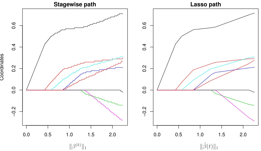
Such greediness, in selecting variable i, is counterbalanced by the small step size > 0; instead of increasing the coefficient ofXi by a (possibly) large amount in the fitted model, forward stagewise only increases it by , which “slows down” the learning process. As a result, it typically requires many iterations to produce estimates of reasonable interest with forward stagewise regression, e.g., it could easily take thousands of iterations to reach a model with only tens of active variables (we use “active” here to refer to variables that are assigned nonzero coefficients). See the left panel of Figure 1 for a small example.
This “slow learning” property is a key difference between forward stagewise regression and the closely-named forward stepwise regressionprocedure: at each iteration, the latter algorithm chooses a variable in a similar manner to that in (2)1, but once it does so, it updates the fitted model by regressing y on all variables selected thus far. While both are greedy algorithms, the stepwise procedure is much greedier; after k iterations, it produces a model with exactly k active variables. Forward stagewise and forward stepwise are old techniques (some classic references for stepwise regression methods are Efroymson, 1966 and Draper and Smith, 1966, but there could have been earlier relevant work). According to Hastie et al. (2009), forward stagewise was historically dismissed by statisticians as being “inefficient” and hence less useful than methods like forward or backward stepwise. This is perhaps understandable, if we keep in mind the limited computational resources of the time. From a modern perspective, however, we now appreciate that “slow learning” is a form of regularization and can present considerable benefits in terms of the generalization error of the fitted models—this is seen not only in regression, but across variety of settings. Furthermore, by modern standards, forward stagewise is computationally cheap: to trace out a path of regularized estimates, we repeat very simple iterations, each one requiring (at most)p inner products, computations that could be trivially parallelized.
The revival of interest in stagewise regression began with the work of Efron et al. (2004), where the authors derived a surprising connection between the sequence of forward stagewise estimates and the solution path of the lasso (Tibshirani, 1996),
ˆ
β(t) = argmin β∈Rp
1
2ky−Xβk 2
2 subject to kβk1≤t, (3) over the regularization parameter t≥0. The relationship between stagewise and the lasso will be reviewed in Section 2.1 in detail, but the two panels in Figure 1 tell the essence
1. IfA denotes the active set at the end of iterationk−1, then at iteration k forward stepwise chooses
the variable isuch that the sum of squared errors from regressing y onto the variables in A∪ {i} is
smallest. This is equivalent to choosingisuch that|XeiT(y−Xβ(k−1))|is largest, whereβ(k−1) denote
the coefficients from regressingyon the variables inA, andXeiis the residual from regressingXion the
0.0 0.5 1.0 1.5 2.0
−0.2
0.0
0.2
0.4
0.6
Stagewise path
Coordinates
kβ(k)k 1
0.0 0.5 1.0 1.5 2.0
−0.2
0.0
0.2
0.4
0.6
Lasso path
kβˆ(t)k1
C
o
or
d
in
at
es
Figure 1: A simple example using the prostate cancer data from Hastie et al. (2009), where the log
PSA score ofn= 67 men with prostate cancer is modeled as a linear function ofp= 8
biological predictors. The left panel shows the forward stagewise regression estimates
β(k)
∈R8,k= 1,2,3, . . ., with the 8 coordinates plotted in different colors. The stagewise
algorithm was run with= 0.01 for 250 iterations, and the x-axis here gives the`1norm
of the estimates across iterations. The right panel shows the lasso solution path, also
parametrized by the`1 norm of the estimate. The similarity between the stagewise and
lasso paths is visually striking; for small enough, they appear identical. This is not a
coincidence and has been rigorously studied by Efron et al. (2004), and other authors; in Section 2.1 we provide an intuitive explanation for this phenomenon.
of the story. The stagewise paths, on the left, appear to be jagged versions of their lasso counterparts, on the right. Indeed, as the step size is made smaller, this jaggedness becomes less noticeable, and eventually the two sets of paths appear exactly the same. This is not a coincidence, and under some conditions (on the problem instance in consideration), it is known that the stagewise path converges to the lasso path, as → 0. Interestingly, when these conditions do not hold, stagewise estimates can deviate substantially from lasso solutions, and yet in such situations the former estimates can still perform competitively with the latter, say, in terms of test error (or really any other standard error metric). This is an important point, and it supports the use of stagewise regression as a general tool for regularized estimation.
1.1 Summary of Our Contributions
This paper departs from the lasso setting and considers the generic convex problem
ˆ
x(t)∈argmin
where f, g : Rn → R are convex functions, and f is differentiable. Motivated by forward
stagewise regression and its connection to the lasso, our main contribution is the
follow-ing general stagewise algorithm for producing an approximate solution path of (4), as the
regularization parametertvaries over [t0,∞). Algorithm 2 (General stagewise procedure)
Fix > 0 and t0 ∈ R. Initialize x(0) = ˆx(t0), a solution in (4) at t = t0. Repeat, for
k= 1,2,3, . . .,
x(k)=x(k−1)+ ∆, (5)
where ∆∈argmin
z∈Rn h∇
f(x(k−1)), zi subject to g(z)≤. (6) The intuition behind the general stagewise algorithm can be seen right away: at each iteration, we update the current iterate in a direction that minimizes the inner product with the gradient of f (evaluated at the current iterate), but simultaneously restrict this direction to be small under g. By applying these updates repeatedly, we implicitly adjust the trade-off between minimizing f and g, and hence one can imagine that thekth iterate
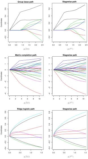
x(k) approximately solves (4) witht=g(x(k)). In Figure 2, we show a few simple examples of the general stagewise paths implemented for various different choices of loss functionsf
and regularizing functions g.
In the next section, we develop further intuition and motivation for the general stage-wise procedure, and we tie in forward stagestage-wise regression as a special case. The rest of this article is then dedicated to the implementation and analysis of stagewise algorithms: Section 3 derives the specific form of the stagewise updates (5), (6) for various problem setups, Section 4 conducts large-scale empirical evaluations of stagewise estimates, Section 5 presents some theory on suboptimality, and Section 6 concludes with a discussion.
Throughout, our arguments and examples are centered around three points, summarized below.
1. Simple, fast estimation procedures. The general framework for stagewise estimation
in Algorithm 2 leads to simple and efficient stagewise procedures for group-structured regularization problems (e.g., the group lasso, multitask learning), trace norm regular-ization problems (e.g., matrix completion), quadratic regularregular-ization problem problems (e.g., nonparametric smoothing), and (some) generalized lasso problems (e.g., image denoising). For such problems, the proposed stagewise procedures are often competi-tive with existing commonly-used algorithms in terms of efficiency, and are generally much simpler.
2. Similar to actual solution paths, but more stable. In many examples, the computed
0.0 0.5 1.0 1.5 2.0 2.5
−0.2
0.0
0.2
0.4
Coordinates
g( ˆβ(t))
0.0 0.5 1.0 1.5 2.0 2.5
−0.2
0.0
0.2
0.4
g(β(k))
C
o
or
d
in
at
es
0 2 4 6 8 10
−4
−3
−2
−1
0
1
2
Matrix completion path
Coordinates
g( ˆβ(t))
0 2 4 6 8 10
−4
−3
−2
−1
0
1
2
Stagewise path
g(β(k))
C
o
or
d
in
at
es
0.0 0.5 1.0 1.5
−0.4
−0.2
0.0
0.2
0.4
0.6
0.8
Ridge logistic path
Coordinates
g( ˆβ(t))
0.0 0.5 1.0 1.5
−0.4
−0.2
0.0
0.2
0.4
0.6
0.8
Stagewise path
g(β(k))
C
o
or
d
in
at
es
Figure 2: Examples comparing the actual solution paths (left column) to the stagewise paths (right column) across various problem contexts, using the prostate cancer data set. The first row considers a group lasso model on the prostate data (where the groups were some-what arbitrarily chosen based on the predictor types); the second row considers a matrix completion task, on a partially observed submatrix of the full predictor matrix; the third row considers a logistic regression model with ridge regularization (the outcome being
3. Competitive statistical performance. Across essentially all cases, even those in which its constructed path is not close to the actual solution path, the stagewise algorithm performs favorably from a statistical point of view. That is, stagewise estimates are comparable to solutions in (4) with respect to relevant error metrics, across various problem settings. This suggests that stagewise estimates deserved to be studied on their own, regardless of their proximity to solutions in (4).
The third point above, on the favorable statistical properties of stagewise estimates, is based on empirical arguments, rather than theoretical ones. Statistical theory for stagewise estimates is an important topic for future work.
2. Properties of the General Stagewise Framework
For motivation and background, we cover the connection between stagewise regression and the lasso in more detail, and then rewrite the stagewise regression updates in a form that naturally suggests the general stagewise proposal of this paper. Following this, we discuss properties of the general stagewise framework, and related work.
2.1 Motivation: Stagewise Regression and the Lasso
The lasso estimator is a popular tool for sparse estimation in the regression setting. Dis-played in (3), we assume for simplicity that the lasso solution ˆβ(t) in (3) is unique, which holds under very weak conditions on X.2 Recall that the parameter t controls the level of sparsity in the estimate ˆβ(t): when t = 0, we have ˆβ(0) = 0, and as t increases, select components of ˆβ(t) become nonzero, corresponding to variables entering the lasso model (nonzero components of ˆβ(t) can also become zero, corresponding to variables leaving the model). The solution path ˆβ(t),t∈[0,∞) is continuous and piecewise linear as a function of t, and for a large enough value oft, the path culminates in a least squares estimate ofy
on X.
The right panel of Figure 1 shows an example of the lasso path, which, as we discussed earlier, appears quite similar to the stagewise path on the left. This is explained by the seminal work of Efron et al. (2004), who describe two algorithms (actually three, but the third is unimportant for our purposes): one for explicitly constructing the lasso path ˆβ(t) as a continuous, piecewise linear function of the regularization parameter t ∈ [0,∞), and another for computing the limiting stagewise regression paths as→0. One of the (many) consequences of their work is the following: if each component of the lasso solution path
ˆ
β(t) is a monotone function of t, then these two algorithms coincide, and therefore so do the stagewise and lasso paths (in the limit as → 0). Note that the lasso paths for the data example in Figure 1 are indeed monotone, and hence the theory confirms the observed convergence of stagewise and lasso estimates in this example.
The lasso has undergone intense study as a regularized regression estimator, and its statistical properties (e.g., its generalization error, or its ability to detect a truly relevant set of variables) are more or less well-understood at this point. Many of these properties cast
2. For example, it suffices to assume thatX has columns in general position, see Tibshirani (2013). Note
that here we are only claiming uniqueness for all parameter values t < t∗, wheret∗ is the smallest`1
the lasso in a favorable light. Therefore, the equivalence between the (limiting) stagewise and lasso paths lends credibility to forward stagewise as a regularized regression procedure: for a small step size , we know that the forward stagewise estimates will be close to lasso estimates, at least when the individual coordinate paths are monotone. At a high level, it is actually somewhat remarkable that such a simple algorithm, Algorithm 1, can produce estimates that can stand alongside those defined by the (relatively) sophisticated optimization problem in (3). There are now several interesting points to raise.
• The nonmonotone case. In practice, the components of the lasso path are rarely
monotone. How do the stagewise and lasso paths compare in such cases? A precise theoretical answer is not known, but empirically, these paths can be quite different. In particular, for problems in which the predictorsX1, . . . Xp are correlated, the lasso coordinate paths can be very wiggly (as variables can enter and leave the model repeatedly), while the stagewise paths are often very stable; see, e.g., Hastie et al. (2007). In support of these empirical findings, the latter authors derived a local characterization of the lasso and forward stagewise paths: they show that at any point along the path, the lasso estimate decreases the sum of squares loss function at an optimal rate with respect to the increase in `1 norm, and the (limiting) forward stagewise estimate decreases the loss function at an optimal rate with respect to the increase in `1 arc length. Loosely speaking, since the `1 arc length accounts for the entire history of the path up until the current point, the (limiting) stagewise algorithm is less “willing” to produce wiggly estimates.
Despite these differences, stagewise estimates tend to perform competitively with lasso estimates in terms of test error, and this is true even with highly correlated predictor variables, when the stagewise and lasso paths are very different (such statements are based on simulations, and not theory; see Hastie et al., 2007; Knudsen, 2013). This is a critical point, as it suggests that stagewise should be considered as an effective tool for regularized estimation, apart from any link to a convex problem. We return to this idea throughout the paper.
• General convex loss functions. Fortunately, the stagewise method extends to sparse
modeling in other settings, beyond Gaussian regression. Let f : Rp → R be a
dif-ferentiable convex loss function, e.g., f(β) = 1
2ky−Xβk 2
2 for the regression setting. Beginning again withβ(0) = 0, the analogy of the stagewise steps in (1), (2) for the present general setting are
β(k)=β(k−1)−·sign ∇if(β(k−1))
·ei, (7)
where i∈argmax j=1,...p |∇
jf(β(k−1))|. (8) That is, at each iteration we update β(k) in the direction opposite to the largest component of the gradient (largest in absolute value). Note that this reduces to the usual update rules (1), (2) whenf(β) = 1
2ky−Xβk 2
2. Rosset et al. (2004) studied the stagewise routine (7), (8), and its connection to the `1-constrained estimate
ˆ
β(t) = argmin β∈Rp
Similar to the result for lasso regression, these authors prove that if the solution ˆβ(t) in (9) has monotone coordinate paths, then under mild conditions3onf, the stagewise paths given by (7), (8) converge to the path ˆβ(t) as→0. This covers, e.g., the cases of logistic regression and Poisson regression losses, with predictor variablesXin general position. The same general message, as in the linear regression setting, applies here: compared to the relatively complex optimization problem (9), the stagewise algorithm (7), (8) is very simple. The most (or really, the only) advanced part of each iteration is the computation of the gradient ∇f(β(k−1)); in the logistic or Poisson regression settings, the components of ∇f(β(k−1)) are given by
∇jf(β(k−1)) =XjT y−µ(β(k−1))
, j= 1, . . . p,
wherey∈Rn is the outcome andµ(β(k−1))∈Rn has components
µi(β(k−1)) = (
1/[1 + exp(−(Xβ(k−1))i)] for logistic regression exp((Xβ(k−1))
i) for Poisson regression
, i= 1, . . . n.
Its precise connection to the `1-constrained optimization problem (9) for monotone paths is encouraging, but even outside of this case, the simple and efficient stagewise algorithm (7), (8) produces regularized estimates deserving of attention in their own right.
• Forward-backward stagewise. Zhao and Yu (2007) examined a novel modification of
forward stagewise, under a general loss function f: at each iteration, their proposal takes a backward step (i.e., moves a component of β(k) towards zero) if this would decrease the loss function by a sufficient amount ξ; otherwise it takes a forward step as usual. The authors prove that, as long as the parameter ξ used for the backward steps scales as ξ = o(), the path from this forward-backward stagewise algorithm converges to the solution path in (9) as → 0. The important distinction here is that their result does not assume monotonicity of the coordinate paths in (9). (It does, however, assume that the loss function f is strongly convex—in the linear regression setting,f(β) = 1
2ky−Xβk 2
2, this is equivalent to assuming thatX∈Rn×p has linearly independent predictors, which requires n≥ p).4 The forward-backward stagewise algorithm hence provides another way to view the connection between (the usual) forward stagewise steps (7), (8) and the `1-regularized optimization problem (9): the forward stagewise path is an approximation to the solution path in (9) given by skipping the requisite backward steps needed to correct for nonmonotonicities.
Clearly, there has been some fairly extensive work connecting the stagewise estimates (1), (2) and the lasso estimate (3), or more generally, the stagewise estimates (7), (8) and
3. Essentially, Rosset et al. (2004) assume that conditions onf that imply a unique solution in (9), and
allow for a second order Taylor expansion of f. Such conditions are thatf(β) =h(Xβ), with htwice
differentiable and strictly convex, andX having columns in general position.
the `1-constrained estimate (9). Still, however, this connection seems mysterious. Both methods produce a regularization path, with a fully sparse model on one end, and a fully dense model on the other—but beyond this basic degree of similarity, why should we expect the stagewise path (7), (8) and the `1 regularization path (9) to be so closely related? The work referenced above gives a mathematical treatment of this question, and we feel, does not provide much intuition. In fact, there is a simple interpretation of the forward stagewise algorithm that explains its connection to the lasso problem, seen next.
2.2 A New Perspective on Forward Stagewise Regression
We start by rewriting the steps (7), (8) for the stagewise algorithm, under a general lossf, as
β(k)=β(k−1)+ ∆, where ∆ =−·sign ∇if(β(k−1))
·ei, and |∇if(β(k−1))|=k∇f(β(k−1))k∞.
As ∇if(β(k−1)) is maximal in absolute value among all components of the gradient, the quantity sign(∇if(β(k−1)))·ei is a subgradient of the`∞ norm evaluated at∇f(β(k−1)):
∆∈ −·∂kxk∞
x=∇f(β(k−1))
.
Using the duality between the`∞ and `1 norms, ∆∈ −·argmax
z∈Rp
h∇f(β(k−1)), zi subject to kzk 1≤1
,
or equivalently,
∆∈argmin z∈Rp h∇
f(β(k−1)), zi subject to kzk1≤.
(Above, as before, the element notation emphasizes that the maximizer or minimizer is not necessarily unique.) Hence the forward stagewise steps (7), (8) satisfy
β(k)=β(k−1)+ ∆, (10)
where ∆∈argmin z∈Rp
h∇f(β(k−1)), zi subject to kzk
1 ≤. (11)
2.3 Basic Properties of the General Stagewise Procedure
Recall the general minimization problem in (4), where we assume that the loss functionf is convex and differentiable, and the regularizergis convex. It can now be seen that the steps (5), (6) in the general stagewise procedure in Algorithm 2 are directly motivated by the forward stagewise steps, as expressed in (10), (11). The explanation is similar to that given above: as we repeat the steps of the algorithm, the iterates are constructed to decrease the loss function f (by following its negative gradient) at the cost of a small increase in the regularizer g. In this sense, the stagewise algorithm navigates the trade-off between minimizingf andg, and produces an approximate regularization path for (4), i.e., the kth iterate x(k) approximately solves problem (4) with t=g(x(k)).
From our work at the end of the last subsection, it is clear that forward stagewise regres-sion (7), (8), or equivalently (10), (11), is a special case of the general stagewise procedure, applied to the `1-regularized problem (9). Moreover, the general stagewise procedure can be applied in many other settings, well beyond `1 regularization, as we show in the next section. Before presenting these applications, we now make several basic remarks.
• Initialization and termination. In many cases, initializing the algorithm is easy: if
g(x) = 0 implies x = 0 (e.g., this is true when g is a norm), then we can start the stagewise procedure att0= 0 andx(0)= 0. In terms of a stopping criterion, a general strategy for (approximately) tracing a full solution path is to stop the algorithm wheng(x(k)) does not change very much between successive iterations. If instead the algorithm has been terminated upon reaching some maximum number of iterations or some maximum value ofg(x(k)), and more iterations are desired, then the algorithm can surely be restarted from the last reached iterate x(k).
• First-order justification. Ifg satisfies the triangle inequality (again, e.g., it would as
a norm), then the increase in the value ofg between successive iterates is bounded by
:
g(x(k))≤g(x(k−1)) +g(∆)≤g(x(k−1)) +.
Furthermore, we can give a basic (and heuristic) justification of the stagewise steps (5), (6). Consider the minimization problem (4) at the parameter t=g(x(k−1)) +; we can write this as
ˆ
x(t)∈argmin x∈Rn
f(x)−f(x(k−1)) subject to g(x)−g(x(k−1))≤,
and then reparametrize as
ˆ
x(t) =x(k−1)+ ∆∗, (12)
∆∗ ∈argmin z∈Rn
f(x(k−1)+z)−f(x(k−1)) subject to g(x(k−1)+z)−g(x(k−1))≤. (13)
We now modify the problem (13) in two ways: first, we replace the objective function in (13) with its first-order (linear) Taylor approximation around x(k−1),
and second, we shrink the constraint set in (13) to
{z∈Rn:g(z)≤} ⊆ {z∈Rn:g(x(k−1)+z)−g(x(k−1))≤},
since, as noted earlier, any element of the left-hand side above is an element of the right-hand side by the triangle inequality. These two modifications define a different update direction
∆∈argmin z∈Rn
h∇f(x(k−1)), zi subject to g(z)≤,
which is exactly the direction (6) in the general stagewise procedure. Hence the stagewise algorithm chooses ∆ as above, rather than choosing the actual direction ∆∗ in (13), to perform an update step fromx(k−1). This update results in a feasible point
x(k)=x(k−1)+ ∆ for the problem (4) att=g(k−1)+; of course, the pointx(k)is not necessarily optimal, but asgets smaller, the first-order Taylor approximation in (14) becomes tighter, so one would imagine that the pointx(k) becomes closer to optimal.
• Dual update form. If g is a norm, then the update direction defined in (6) can be
expressed more succinctly in terms of the dual norm g∗(x) = maxg(z)≤1xTz. We write
∆∈ −·argmax z∈Rn h∇
f(x(k−1)), zi subject to g(z)≤1 =−·∂g∗ ∇f(x(k−1))
, (15)
i.e., the direction ∆ is − times a subgradient of the dual norm g∗ evaluated at
∇f(x(k−1)). This is a useful observation, since many norms admit a known dual norm with known subgradients; we will see examples of this in the coming section.
• Invariance around ∇f. The level of difficulty associated with computing the update
direction, i.e., in solving problem (6), depends entirely on g and not on f at all (assuming that∇f can be readily computed). We can think of ∆ as an operator on
Rn:
∆(x)∈argmin z∈Rn
hx, zi subject to g(z)≤. (16)
This operator ∆(·) is often called the linear minimization oracle associated with the functiong, in the optimization literature. At each inputx, it returns a minimizer of the problem in (16). Provided that ∆(·) can be expressed in closed-form—which is fortuitously the case for many common statistical optimization problems, as we will see in the sections that follow—the stagewise update step (5) simply evaluates this operator at∇f(x(k−1)), and adds the result tox(k−1):
x(k)=x(k−1)+ ∆ ∇f(x(k−1))
.
• Unbounded stagewise steps. Suppose that g is a seminorm, i.e., it satisfies g(ax) =
|a|g(x) for a∈R, and g(x+y)≤g(x) +g(y), butg can have a nontrivial null space,
Ng = {x ∈ Rn : g(x) = 0}. In this case, the stagewise update step in (5) can be
unbounded; in particular, if
h∇f(x(k)), zi 6= 0 for somez∈Ng, (17) then we can drive h∇f(x(k)), zi → −∞ along a sequence with g(z) = 0, and so the stagewise update step would be clearly undefined. Fortunately, a simple modification of the general stagewise algorithm can account for this problem. Since we are assuming thatgis a seminorm, the setNgis a linear subspace. To initialize the general stagewise algorithm at say t0 = 0, therefore, we solve the linearly constrained optimization problem
x(0)∈argmin x∈Ng
f(x).
In subsequent stagewise steps, we then restrict the updates to lie in the subspace orthogonal to Ng. That is, to be explicit, we replace (5) (6) in Algorithm 2 with
x(k)=x(k−1)+ ∆, (18)
where ∆∈argmin z∈N⊥
g
h∇f(x(k−1)), zi subject to g(z)≤, (19)
where Ng⊥ denotes the orthocomplement of Ng. We will see this modification, e.g., put to use for the quadratic regularizerg(β) =βTQβ, whereQis positive semidefinite and singular.
Some readers may wonder why we are working with the constrained problem (4), and not
ˆ
x(λ)∈argmin x∈Rn
f(x) +λg(x), (20)
where λ ≥ 0 is now the regularization parameter, and is called the Lagrange multiplier associated with g. It is probably more common in the current statistics and machine learning literature for optimization problems to be expressed in the Lagrange form (20), rather than the constrained form (4). The solution paths of (4) and (20) (given by varying
tand λin their respective problems) are not necessarily equal for general convex functions
f and g; however, they are equal under very mild assumptions5, which hold for all of the examples visited in this paper. Therefore, there is not an important difference in terms of studying (4) versus (20). We choose to focus on (4) as we feel that the intuition for stagewise algorithms is easier to see with this formulation.
2.4 Related Work
There is a lot of work related to the proposal of this paper. Readers familiar with opti-mization will likely identify the general stagewise procedure, in Algorithm 2, as a particular
5. For example, it is enough to assume thatg≥0, and that for all parameterst, λ≥0, the solution sets of
type of (normalized) steepest descent. Steepest descent is an iterative algorithm for mini-mizing a smooth convex function f, in which we update the current iterate in a direction that minimizes the inner product with the gradient off (evaluated at the current iterate), among all vectors constrained to have norm k · k bounded by 1 (e.g., see Boyd and Van-denberghe, 2004); the step size for the update can be chosen in any one of the usual ways for descent methods. Note that gradient descent is simply a special case of steepest descent
with k · k = k · k2 (modulo normalizing factors). Meanwhile, the general stagewise
algo-rithm is just steepest descent with k · k=g(·), and a constant step size . It is important to point out that our interest in the general stagewise procedure is different from typical interest in steepest descent. In the classic usage of steepest descent, we seek to minimize a differentiable convex functionf; our choice of normk · k affects the speed with which we can find such a minimizer, but under weak conditions, any choice of norm will eventually bring us to a minimizer nonetheless. In the general stagewise algorithm, we are not really interested in the final minimizer itself, but rather, the path traversed in order to get to this minimizer. The stagewise path is composed of iterates that have interesting statistical properties, given by gradually balancing f and g; choosing different functions g will lead to generically different paths. Focusing on the path, instead of its endpoint, may seem strange to a researcher in optimization, but it is quite natural for researchers in statistics and machine learning.
Another method related to our general stagewise proposal is theFrank-Wolfe algorithm
(Frank and Wolfe, 1956), used to minimize a differentiable convex functionf over a convex set C. Similar to (projected) gradient descent, which iteratively minimizes local quadratic approximations of f over C, the Frank-Wolfe algorithm iteratively minimizes local linear approximations of f overC. In a recent paper, Jaggi (2013) shed light on Frank-Wolfe as an efficient, scalable algorithm for modern machine learning problems. For a single value of the regularization parameter t, the Frank-Wolfe algorithm can be used to solve problem (4), taking as the constraint set C ={x :g(x)≤t}; the Frank-Wolfe steps here look very similar to the general stagewise steps (5), (6), but an important distinction is that the iterates from Frank-Wolfe result in a single estimate, rather than each iterate constituting its own estimate along the regularization path, as in the general stagewise procedure. This connection deserves more discussion, see Online Appendix A.1. Other well-known methods based on local linearization are cutting-plane methods (Kelley, 1960) and bundle methods
(Hiriart-Urruty and Lemarechal, 1993). Teo et al. (2007) present a general bundle method for regularized risk minimization that is particularly relevant to our proposal (see also Teo et al., 2010); this is similar to the Frank-Wolfe approach in that it solves the problem (4) at a fixed value of the parameter t (one difference is that its local linearization steps are based on the entire history of previous iterates, instead of just the single last iterate). For brevity, we do not conduct a detailed comparison between their bundle method and our general stagewise procedure, though we believe it would be interesting to do so.
methods, gradient boosting (Friedman, 2001) most closely parallels forward stagewise fit-ting. Consider a setup in which our weak learners are the individual predictor variables
X1, . . . Xp, and the loss function is L(Xβ) =f(β). The gradient boosting updates, using a shrinkage factor, are most commonly expressed in terms of the fitted values, as in
Xβ(k)=Xβ(k−1)+·αiXi, (21)
where αi ∈argmin α∈R
L(Xβ(k−1)+αXi), (22)
and i∈argmin j=1,...p
min
α∈R k − ∇L(Xβ
(k−1))
−αXjk22
. (23)
The step (23) selects the weak learnerXithat best matches the negative gradient,−∇L(Xβ(k−1)), in a least squares sense; the step (22) chooses the coefficient αi ofXi via line search. If we assume that the variables have been scaled to have unit norm, kXjk2 = 1 for j = 1, . . . p, then it is easy to see that (23) is equivalent to
i∈argmax j=1,...p |
XjT∇L(Xβ(k−1))|= argmax j=1,...p |∇j
f(β(k−1))|,
which is exactly the same selection criterion used by forward stagewise under the loss function f, as expressed in (8). Therefore, at a given iteration, gradient boosting and forward stagewise choose the next variable i in the same manner, and only differ in their choice of the coefficient of Xi in the constructed additive model. The gradient boosting update in (21) adds·αiXi to the current model, whereαi is chosen by line search in (22); meanwhile, the forward stagewise update in (7) can be expressed as
Xβ(k)=Xβ(k−1)+·siXi, (24)
where si = −sign(∇if(β(k−1)), a simple choice of coefficient compared to αi. Because αi is chosen by minimizing the loss function along the direction defined by Xi (anchored at
Xβ(k−1)), gradient boosting is even more greedy than forward stagewise, but practically there is not a big difference between the two, especially when is small. In fact, the distinction between (21) and (24) is slight enough that several authors refer to forward stagewise as a boosting procedure, e.g., Rosset et al. (2004), Zhao and Yu (2007), and Buhlmann and Yu (2010) refer to forward stagewise as -boosting.
based on the regularizer g, through the definition of ∆ in (6). Such weak learners seem intuitively reasonable in various problem settings: they end up being groups of variables for group-structured estimation problems (see Section 3.1), rank 1 matrices for matrix completion (Section 3.3), and pixel contrasts for image denoising (Section 3.5). This may lead to an interesting perspective on gradient boosting with an arbitrary regularization scheme, though we do not explore it further.
Finally, the form of the update ∆ in (6) sets our work apart from other general path tracing procedures. Zhao and Yu (2007) and Friedman (2008) propose approximate path following methods for optimization problems whose regularizers extend beyond the`1norm, but their algorithms only update one component of the estimate at a time (which corre-sponds to using individual variables as weak learners, in the boosting perspective); on the other hand, our general stagewise procedure specifically adapts its updates to the regu-larizer of concern g. We note that, in certain special cases (i.e., for certain regularizers
g), our proposed algorithm bears similarities to existing algorithms in the literature: for ridge regularization, our proposal is similar to gradient-directed path following, as studied in Friedman and Popescu (2004) and Ramsay (2005), and for`1/`2 multitask learning, our stagewise algorithm is similar to the block-wise path following method of Obozinski et al. (2010).
3. Applications of the General Stagewise Framework
In each subsection below, we walk through the application of the stagewise framework to a particular type of regularizer.
3.1 Group-structured Regularization
We begin by considering the group-structured regularization problem
ˆ
β(t)∈argmin β∈Rp
f(β) subject to G X
j=1
wjkβIjk2 ≤t, (25)
where the index set {1, . . . p} has been partitioned into G groups I1, . . .IG, βIj ∈ R
pj
denotes the components of β ∈Rp for thejth group, andw1, . . . wG≥0 are fixed weights. The lossf is kept as a generic differentiable convex function—this is because, as explained in Section 2.3, the stagewise updates are invariant around∇f, in terms of their computational form.
Note that the group lasso problem (Bakin, 1999; Yuan and Lin, 2006) is a special case of (25). In the typical group lasso regression setup, we observe an outcome y ∈ Rn and
predictors X ∈Rn×p, and the predictor variables admit some natural grouping I1, . . .IG. To perform group-wise variable selection, one can use the group lasso estimator, defined as in (25) with
f(β) = 1 2 y−
G X
j=1
XIjβIj
2
2 and wj =
√p
whereXIj ∈Rn×pj is the predictor matrix for groupj, andpj =|Ij|is the size of the group
j. The same idea clearly applies outside of the linear regression setting (e.g., see Meier et al., 2008 for a study of the group lasso regularization in logistic regression).
A related yet distinct problem is that of multitask learning. In this setting we consider not one but multiple learning problems, or tasks, and we want to select a common set of variables that are important across all tasks. A popular estimator for this purpose is based on `1/`2 regularization (Argyriou et al., 2006; Obozinski et al., 2010), and also fits into the framework (25): the loss function f becomes the sum of the losses across the tasks, and the groupsI1, . . .IG collect the coefficients corresponding to the same variables across tasks. For example, in multitask linear regression, we write y(i) ∈
Rn for the outcome,
X(i) ∈
Rn×m for the predictors, and β(i) the coefficients for the ith task, i= 1, . . . r. We
form a global coefficient vectorβ = (β(1), . . . β(m))∈
Rp, where p=m·r, and form groups I1, . . .Im, where Ij collects the coefficients of predictor variable j across the tasks. The
`1/`2 regularized multitask learning estimator is then defined as in (25) with
f(β) = 1 2
r X
i=1
ky(i)−X(i)β(i)k2
2 and wj = 1, j = 1, . . . m,
where the default is to set all of the weights to 1, in the lack of any prior information about variable importance (note that the groups I1, . . .Im are all the same size here).
The general stagewise algorithm, Algorithm 2, does not make any distinction between cases such as the group lasso and multitask learning problems; it only requires f to be a convex and smooth function. To initialize the algorithm for the group regularized problem (25), we can take t0 = 0 and β(0) = 0. The next lemma shows how to calculate the appropriate update direction ∆ in (6).
Lemma 1 For g(β) =PG
j=1wjkβIjk2, the general stagewise procedure in Algorithm 2
re-peats the updates β(k) =β(k−1)+ ∆, where ∆can be computed as follows: first find i such
that
k(∇f)Iik2 wi
= max j=1,...G
k(∇f)Ijk2 wj
, (26)
where we abbreviate ∇f =∇f(β(k−1)), then let
∆Ij = 0 for all j6=i, (27)
∆Ii =
−·(∇f)Ii wik(∇f)Iik2
. (28)
We omit the proof; it follows straight from the KKT conditions for (6), with g as defined in the lemma. Computation of ∆ in (26), (27), (28) is very cheap, and requires
O(p) operations. To rephrase: at thekth iteration, we simply find the group i such that the corresponding block of the gradient ∇f(β(k−1)) has the largest `
match our intuition about the role of the constraint in (25)—for some select groups, all coefficients are set to nonzero values, and for other groups, all coefficients are set to zero. That the actual solution in (25) satisfies this intuitive property can be verified by examining its own KKT conditions.
Looking back at Figure 2, the first row compares the exact solution and stagewise paths for a group lasso regression problem. The stagewise path was computed using 300 steps with= 0.01, and shows strong similarities to the exact group lasso path. In other problem instances, say, when the predictors across different groups are highly correlated, the group lasso coefficient paths can behave wildly with t, and yet the stagewise paths can appear much less wild and more stable. Later, in Section 4, we consider larger examples and give more thorough empirical comparisons.
3.2 Group-structured Regularization with Arbitrary Norms
Several authors have considered group-based regularization using the `∞ norm in place of the usual`2 norm (e.g., see Turlach et al., 2005 for such an approach in multitask learning). To accommodate this and other general group-structured regularization approaches, we consider the problem
ˆ
β(t)∈argmin β∈Rp
f(β) subject to G X
j=1
wjhj(βIj)≤t, (29)
where eachhjis an arbitrary norm. Leth∗j denote the dual norm ofhj; e.g., ifhj(x) =kxkqj,
thenh∗j(x) =kxkrj, where 1/qj+ 1/rj = 1. Similar to the result in Lemma 1, the stagewise
updates for problem (29) take a simple group-based form.
Lemma 2 For g(β) =PG
j=1wjhj(βIj), the general stagewise procedure in Algorithm 2
re-peats the updates β(k) =β(k−1)+ ∆, where ∆can be computed as follows: first find i such
that
h∗i (∇f)Ii
wi
= max j=1,...G
h∗j (∇f)Ij
wj
,
where we abbreviate ∇f =∇f(β(k−1)), then let
∆Ij = 0 for all j6=i,
∆Ii ∈ − wi ·
∂h∗i (∇f)Ii
.
Again we omit the proof; it follows from the KKT conditions for (6). Indeed, Lemma 2 covers Lemma 1 as a special case, recalling that the `2 norm is self-dual. Also, recalling that the `∞ and `1 norms are dual, Lemma 2 says that the stagewise algorithm forg(β) = PG
j=1wjkβIjk∞ first finds isuch that
k(∇f)Iik1 wi
= max j=1,...G
k(∇f)Ijk1 wj
and then defines the update direction ∆ by
∆Ij = 0 for all j6=i,
∆`=−
wi ·
(
0 for `∈ Ii,(∇f)` = 0 sign (∇f)`
for `∈ Ii,(∇f)` 6= 0.
More broadly, Lemma 2 provides a general prescription for deriving the stagewise updates for regularizers that are block-wise sums of norms, as long as we can compute subgradients of the dual norms. For example, the norms in consideration could be a mix of `p norms, matrix norms, etc.
3.3 Trace Norm Regularization
Consider a class of optimization problems over matrices,
ˆ
B(t)∈ argmin B∈Rm×n
f(B) subject to kBk∗ ≤t, (30)
wherekBk∗denotes the trace norm (also called the nuclear norm) of a matrixB, i.e., the sum
of its singular values. Perhaps the most well-known example of trace norm regularization comes from the problem ofmatrix completion(e.g., see Candes and Recht, 2009; Candes and Tao, 2010; Mazumder et al., 2010). Here the setup is that we only partially observe entries of a matrix Y ∈Rm×n—say, we observe all entries (i, j)∈Ω—and we seek to estimate the
missing entries. A natural estimator for this purpose (studied by, e.g., Mazumder et al., 2010) is defined as in (30) with
f(B) = 1 2
X
(i,j)∈Ω
(Yij −Bij)2.
The trace norm also appears in interesting examples beyond matrix completion. For exam-ple, Chen and Ye (2014) consider regularization with the trace norm in multiple nonpara-metric regression, and Harchaoui et al. (2012) consider it in large-scale image classification. The general stagewise algorithm applied to the trace norm regularization problem (30) can be initialized witht0 = 0 and B(0) = 0, and the update direction in (6) is now simple and efficient.
Lemma 3 For g(B) = kBk∗, the general stagewise procedure in Algorithm 2 repeats the
updates β(k)=β(k−1)+ ∆, where
∆ =−·uvT, (31)
with u, v being leading left and right singular vectors, respectively, of ∇f(B(k−1)).
The proof relies on the fact that the dual of the trace norm g(B) =kBk∗ is the spectral
A=∇f(B(k−1)), we first run the power method on the m×m matrixAAT, or the n×n matrix ATA, depending on whichever is smaller. This gives us either u or v; to recover the other, we then simply use matrix multiplication: v =ATu/kATuk
2 or u=Av/kAvk2. The power method is especially efficient if A=∇f(B(k−1)) is sparse (each iteration being faster), or has a large spectral gap (fewer iterations required until convergence). Of course, alternatives to the power method can be used for computing the leading singular vectors of ∇f(B(k−1)), such as methods based on inverse iterations, Rayleigh quotients, or QR iterations; see, e.g., Golub and Van Loan (1996).
In the second row of Figure 2, the exact and stagewise paths for are shown matrix completion problem, where the stagewise paths were computed using 500 steps with = 0.05. While the two sets of paths appear fairly similar, we note that it is harder to judge the degree of similarity between the two in the matrix completion context. Here, the coordinate paths correspond to entries in the estimated matrix ˆB, and their roles are not as clear as they are in, say, in a regression setting, where the coordinate paths correspond to the coefficients of individual variables. In other words, it is difficult to interpret the slight differences between the exact and stagewise paths in the second row of Figure 2, which present themselves as the trace norm grows large. Therefore, to get a sense for the effect of these differences, we might compare the mean squared error curves generated by the exact and stagewise estimates. This is done in depth in Section 4.
3.4 Quadratic Regularization Consider problems of the form
ˆ
β(t)∈argmin β∈Rp
f(β) subject to βTQβ≤t, (32)
whereQ0, a positive semidefinite matrix. The quadratic regularizer in (32) encompasses several common statistical tasks. WhenQ=I, the regularization termβTβ=kβk2
2 is well-known as ridge (Hoerl and Kennard, 1970), or Tikhonov regularization (Tikhonov, 1943). This regularizer shrinks the components of the solution ˆβ towards zero. In a (generalized) linear model setting with many predictor variables, such shrinkage helps control the variance of the estimated coefficients. Beyond this simple ridge case, roughness regularization in nonparametric regression often fits into the form (32), with Q not just the identity. For example,smoothing splines(Wahba, 1990; Green and Silverman, 1994) andP-splines(Eilers and Marx, 1996) can both be expressed as in (32). To see this, suppose thaty1, . . . yn ∈R
are observed across input points x1, . . . xn ∈R, and let b1, . . . bp denote the B-spline basis (of, say, cubic order) with knots at locationsz1, . . . zp ∈R. Smoothing splines use the inputs
as knots,z1 =x1, . . . zp =xn (so that p=n); P-splines typically employ a (much) smaller number of knots across the range of x1, . . . xn ∈ R. Both estimators solve problem (32),
with a loss function f(β) = 1
2ky−Bβk 2
2, and B ∈ Rn×p having entries Bij = bj(xi), but the two use a different definition forQ: its entries are given byQij =
R
When Q is positive definite, the general stagewise algorithm, applied to (32), can be initialized with t0 = 0 and β(0) = 0. The update direction ∆ in (6) is described by the following lemma.
Lemma 4 For g(β) = βTQβ, with Q a positive definite matrix, the general stagewise
procedure in Algorithm 2 repeats the updates β(k)=β(k−1)+ ∆, where
∆ =−√· Q
−1∇f p
(∇f)TQ−1∇f, (33)
and ∇f is an abbreviation for ∇f(β(k−1)).
The proof follows by checking the KKT conditions for (6). When Q = I, the update step (33) of the general stagewise procedure for quadratic regularization is computationally trivial, reducing to
∆ =−√· ∇f k∇fk2
.
This yields fast, simple updates for ridge regularized estimators. For a general matrix Q, computing the update direction in (33) boils down to solving the linear equation
Qv=∇f(β(k−1)) (34)
in v. This is expensive for an arbitrary, denseQ; a single solve of the linear system (34) generally requiresO(p3) operations. Of course, since the systems across all iterations involve the same linear operator Q, we could initially compute a Cholesky decomposition of Q
(or a related factorization), requiring O(p3) operations, and then use this factorization to solve (34) at each iteration, requiring only O(p2) operations. While certainly more efficient than the naive strategy of separately solving each instance of (34), this is still not entirely desirable for large problems.
On the other hand, for several cases in whichQis structured or sparse, the linear system (34) can be solved efficiently. For example, ifQ is banded with bandwidth d, then we can solve (34) in O(pd2) operations (actually, an initial Cholesky decomposition takes O(pd2) operations, and each successive solve with this decomposition then takesO(pd) operations). Importantly, the matrix Q is banded in both the smoothing spline and P-spline regu-larization cases: for smoothing splines, Q is banded because the B-spline basis functions have local support; for P-splines, Q is banded because the discrete difference operator is. However, some care must be taken in applying the stagewise updates in these cases, as
Q is singular, i.e., positive semidefinite but not strictly positive definite. The stagewise algorithm needs to be modified, albeit only slightly, to deal with this issue—this modifica-tion was discussed in (18), (19) in Secmodifica-tion 2.3, and here we summarize the implicamodifica-tions for problem (32). First we compute the initial iterate to lie in null(Q), the null space ofQ,
β(0)∈ argmin β∈null(Q)
f(β). (35)
of order k−1. The stagewise algorithm is then initialized at such a point β(0) in (35), andt0 = 0. For future iterations, note that when∇f(β(k)) has a nontrivial projection onto null(Q), the stagewise update in (6) is undefined, sinceh∇f(β(k)), zican be made arbitrarily small along a direction z such that zTQz = 0. Therefore, we must further constrain the stagewise update to lie in the orthocomplement null(Q)⊥= row(Q), the row space ofQ, as in
∆∈ argmin z∈row(Q)h∇
f(β(k−1)), zi subject to zTQz≤. It is not hard to check that, instead of (33), the update now becomes
∆ =−√· Q
+∇f p
(∇f)TQ+∇f, (36) withQ+ denoting the (Moore-Penrose) generalized inverse of Q.
From a computational perspective, the stagewise update in (36) for the rank deficient case does not represent more much work than that in (33) for the full rank case. With P-splines, e.g., we haveQ=DTDwhereD∈
R(n−k)×nis a banded matrix of full row rank.
A short calculation shows that in this case
(DTD)+=DT(DDT)−2D,
i.e., applying Q+ is computationally equivalent to two banded linear system solves and two banded matrix multiplications. Hence one stagewise update for P-spline regularization problems takes O(p) operations (the bandwidth of D is a constant, d=k+ 1), excluding computation of the gradient.
The third row of Figure 2 shows an example of logistic regression with ridge regular-ization, and displays the grossly similar exact solution and stagewise paths. Notably, the stagewise path here was constructed using only15 steps, with an effective step size√= 0.1. This is a surprisingly small number of steps, especially compared to the numbers needed by stagewise in the examples (both small and large) from other regularization settings covered in this paper. As far as we can tell, this rough scaling appears to hold for ridge regular-ization problems in general—for such problems, the stagewise algorithm can be run with relatively large step sizes for small numbers of steps, and it will still produce statistically appealing paths. Unfortunately, this trend does not persist uniformly across all quadratic regularization problems; it seems that the ridge case (Q=I) is really a special one.
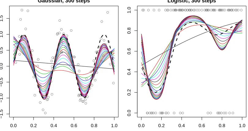
parameter value. The example is instead meant to portray that the stagewise algorithm can produce smooth and visually reasonable estimates of the underlying curve.
The right panel of Figure 3 displays an analogous example using n = 100 binary ob-servations, y1, . . . y100, generated according to the probabilities p∗i = 1/(1 +e−µ(xi)), i = 1, . . .100, where the inputsx1, . . . x100were sampled uniformly from [0,1], andµis a smooth function. The probability curvep∗(x) = 1/(1 +e−µ(x)) is drawn as a thick dotted black line. We ran the stagewise algorithm under a logistic loss, with √= 0.005, and for 300 steps; the figure plots the probability curves associated with the stagewise estimates (from ev-ery 15th step along the path, for visibility). Again, we can see that the fitted curves are smooth and visually reasonable. Computationally, the difficulty of the stagewise algorithm in this logistic setting is essentially the same as that in the previous Gaussian setting; all that changes is the computation of the gradient, which is an easy task. The exact solution, however, is more difficult to compute in this setting than the previous, and requires the use of iterative algorithm like Newton’s method. This kind of computational invariance around the loss function, recall, is an advantage of the stagewise framework.
● ● ● ● ● ● ● ● ● ● ● ● ● ● ● ● ● ● ● ● ● ● ● ● ● ● ● ●● ●● ● ● ● ● ● ● ● ●● ● ●●● ● ● ● ● ● ●● ● ● ● ● ● ●● ● ● ●● ● ● ● ● ●● ● ● ● ● ● ● ● ● ● ● ● ● ● ● ● ● ● ● ● ●● ● ● ● ● ● ● ● ● ● ● ●
0.0 0.2 0.4 0.6 0.8 1.0
−1.5 −1.0 −0.5 0.0 0.5 1.0 1.5
Gaussian, 300 steps
●● ●● ● ●●●● ● ● ● ●●●●● ● ● ● ●● ● ●● ● ● ●●●●●●●● ● ●●● ● ●●●●●●●●●●●●●●●● ● ●●●●● ● ●● ● ●●●●●● ●● ●● ● ●●● ● ●● ● ● ● ● ●● ● ●●●● ● ●●●● ●
0.0 0.2 0.4 0.6 0.8 1.0
0.0 0.2 0.4 0.6 0.8 1.0
Logistic, 300 steps
Figure 3: Snapshots of the stagewise path for P-spline regularization problems, with continuous data in the left panel, and binary data in the right panel. In both examples, we use
n= 100 points, and the true data generating curve is displayed as a thick dotted black
line. The colored curves show the stagewise estimates over the first 300 path steps (plotted are every 15th estimate, for visibility).
3.5 Generalized Lasso Regularization
In this last application, we study generalized`1 regularization problems, ˆ
β(t)∈argmin β∈Rp
where D is a given matrix (it need not be square). The regularization term above is also calledgeneralized lassoregularization, since it includes lasso regularization as a special case, withD=I, but also covers a number of other regularization forms (Tibshirani and Taylor, 2011). For example, fused lasso regularization is encompassed by (37), with D chosen to be the edge incidence matrix of some graphG, having nodes V ={1, . . . p} and edges E=
{e1, . . . em}. In the special case of the chain graph, whereinE ={{1,2},{2,3}, . . .{p−1, p}}, we have
D=
−1 1 0 . . . 0 0
0 −1 1 . . . 0 0 ..
.
0 0 0 . . . −1 1
,
so that kDβk1 =Pj=1p−1|βj−βj+1|. This regularization term encourages the ordered com-ponents of β to be piecewise constant, and problem (37) with this particular choice of D
is usually called the1-dimensional fused lasso in the statistics literature (Tibshirani et al., 2005), or 1-dimensional total variation denoisingin signal processing (Rudin et al., 1992). In general, the edge incidence matrixD∈Rm×p has rows corresponding to edges inE, and
its `th row is
D` = (0, . . .−1
↑
i
, . . .1
↑
j
, . . .0)∈Rp,
provided that the`th edge ise` ={i, j}. HencekDβk1 =P{i,j}∈E|βi−βj|, a regularization term that encourages the components of β to be piecewise constant with respect to the structure defined by the graphG. Higher degrees of smoothness can be regularized in this framework as well, usingtrend filteringmethods; see Kim et al. (2009) or Tibshirani (2014) for the 1-dimensional case, and Wang et al. (2015) for the more general case over arbitrary graphs.
Unfortunately the stagewise update in (6), under the regularizer g(β) = kDβk1, is not computationally tractable. Computing this update is the same as solving a linear program, absent of any special structure in the presence of a generic matrix D. But we can make progress by studying the generalized lasso from the perspective of convex duality. Our jumping point for the dual is actually the Lagrange form of problem (37), namely
ˆ
β(λ)∈argmin β∈Rp
f(β) +λkDβk1, (38)
with λ≥0 now being the regularization parameter. The switch from (37) to (38) is justi-fied because the two parametrizations admit identical solution paths. Following standard arguments in convex analysis, the dual problem of (38) can be written as
ˆ
u(λ)∈argmin u∈Rm
f∗(−DTu) subject to kuk∞≤λ, (39)
with f∗ denoting the convex conjugate of f. The primal and dual solutions satisfy the relationship
primal solution path via (40). The stagewise procedure for (39) can be initialized with
λ0 = 0 and u(0) = 0, and the form of the updates is described next. We assume that the conjugate functionf∗ is differentiable, which holds iff is strictly convex.
Lemma 5 Applied to the problem (39), the general stagewise procedure in Algorithm 2
repeats the updates u(k)=u(k−1)+ ∆, where
∆i =−·
1
D∇f∗(−DTu(k−1)) i <0
−1
D∇f∗(−DTu(k−1)) i >0
0
D∇f∗(−DTu(k−1)) i = 0
for i= 1, . . . m. (41)
The proof follows from the duality of the `∞ and `1 norms, and the alternative repre-sentation in (15) for stagewise updates. Computation of ∆ in (41), aside from evaluating the gradient ∇f∗, reduces to two matrix multiplications: one by D and one by DT. In many cases (e.g., fused lasso and trend filtering problems), the matrix D is sparse, which makes this update step very cheap. To reiterate the dual strategy: we compute the dual estimatesu(k),k= 1,2,3, . . . using the stagewise updates outlined above, and we compute primal estimates β(k),k= 1,2,3, . . . by solving for β(k) in the stationarity condition
∇f(β(k)) +DTu(k) = 0, (42)
for each k. The kth dual iterateu(k) is viewed as an approximate solution in (39) at λ=
ku(k)k
∞, and thekth primal iterateβ(k) an approximate solution in (37) att=kDβ(k)k1. As pointed out by a referee of this paper, there is a key relationship between f and its conjugate f∗ that simplifies the update direction in (41) considerably. At step k, observe that
∇f∗(−DTu(k−1)) =∇f∗(∇f(β(k−1))) =β(k−1).
The first equality comes from the primal-dual relationship (40) at step k−1, and the second is due to the fact that x=∇f∗(z) ⇐⇒ z=∇f(x). As a result, the dual update u(k)=u(k−1)+ ∆ with ∆ as in (41) can be written more succinctly as
u(k) =u(k−1)−·sign(Dβ(k−1)), (43) where sign(·) is to be interpreted componentwise (with the convention sign(0) = 0). There-fore, one can think of the dual stagewise strategy as alternating between computing a dual estimate u(k) as in (43), and computing a primal estimateβ(k) by solving (42).
We note that, since the stagewise algorithm is being run through the dual, the estimates
β(k),k = 1,2,3, . . . for generalized lasso problems differ from those in the other stagewise implementations encountered thus far, in that β(k), k = 1,2,3, . . . correspond to approxi-mate solutions atincreasing levels of regularization, as kincreases. That is, the stagewise algorithm for problem (37) begins at the unregularized end of the path and iterates towards the fully regularized end, which is opposite to its usual direction.
A special case worth noting is that of Gaussian signal approximator problems, where the loss is f(β) = 1
2ky−βk 2
2. For such problems, the primal-dual relationship in (42) reduces to
for each k. This means that the initializationu(0) = 0 and λ
0 = 0 in the dual is the same asβ(0) =y and t
0 =kDyk1 in the primal. Furthermore, it means that the dual updates in (43) lead to primal updates that can be expressed directly as
β(k) =β(k−1)−·DTsign(Dβ(k−1)). (44) From the pure primal perspective, therefore, the stagewise algorithm begins with the trivial unregularized estimateβ(0) =y, and to fit subsequent estimates in (44), it iteratively shrinks along directions opposite to the active rows of D. That is, if D`β(k−1) > 0 (where D` is the `th row of D), then the algorithm adds DT
` to β(k−1) in forming β(k), which shrinks
D`β(k) towards zero, asD`D`T >0 (recall that D` is a row vector). The caseD`β(k−1)<0 is similar. IfD`β(k−1) = 0, then no shrinkage is applied alongD`.
This story can be made more concrete for fused lasso problems, whereDis the edge inci-dence matrix of a graph: here the update in (44) evaluates the differences across neighboring components ofβ(k−1), and for any nonzero difference, it shrinks the associated components towards each other to build β(k). The level of shrinkage is uniform across all active differ-ences, as any two neighboring components move a constant amounttowards each other.6 This is a simple and natural iterative procedure for fitting piecewise constant estimates over graphs. For small examples using 1d and 2d grid graphs, see Online Appendix A.3.
4. Large-scale Examples and Practical Considerations
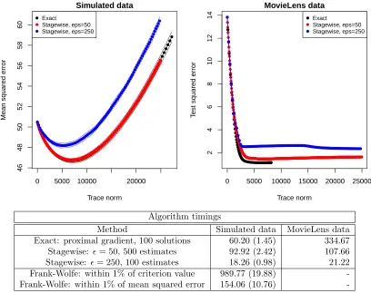
We compare the proposed general stagewise procedure to various alternatives, with respect to both computational and statistical performance, across the three of the four major reg-ularization settings seen so far. The fourth setting is moved to Online Appendix A.4 for reasons of space. The current section specifically investigates large examples, at least rela-tive to the small examples presented in Sections 1–3. Of course, one can surely find room to criticize our comparisons, e.g., with respect to a different tuning of the algorithm that computes exact solutions, a coarser grid of regularization parameter values over which it computes solutions, a different choice of algorithm completely, etc. We have tried to con-duct fair comparisons in each problem setting, but we recognize that perfectly fair and exhaustive comparisons are near impossible. The message that we hope to convey is not that the stagewise algorithm is computationally superior to other algorithms in the prob-lems we consider, but rather, that the stagewise algorithm is computationally competitive with the others, yet it is very simple, and capable of producing estimates of high statistical quality.
4.1 Group Lasso Regression
Overview. We examine two simulated high-dimensional group lasso regression problems. To compute group lasso solution paths, we used theSGLR package, available on the CRAN repository. This package implements a block coordinate descent algorithm for solving the group lasso problem, where each block update itself applies accelerated proximal gradient
6. This is assuming thatD is the edge incidence matrix of an unweighted graph; with edge weights, the
rows ofD scale accordingly, and so the effective amounts of shrinkage in the stagewise algorithm scale