Revisiting Bayesian Blind Deconvolution
David Wipf [email protected]
Visual Computing Group Microsoft Research
Building 2, No. 5 Danling Street Beijing, P.R. China, 100080
Haichao Zhang [email protected]
School of Computer Science
Northwestern Polytechnical University 127 West Youyi Road
Xi’an, P.R. China, 710072
Editor:Lawrence Carin
Abstract
Blind deconvolution involves the estimation of a sharp signal or image given only a blurry observation. Because this problem is fundamentally ill-posed, strong priors on both the sharp image and blur kernel are required to regularize the solution space. While this naturally leads to a standard MAP estimation framework, performance is compromised by unknown trade-off parameter settings, optimization heuristics, and convergence issues stemming from non-convexity and/or poor prior selections. To mitigate some of these problems, a number of authors have recently proposed substituting a variational Bayesian (VB) strategy that marginalizes over the high-dimensional image space leading to better estimates of the blur kernel. However, the underlying cost function now involves both in-tegrals with no closed-form solution and complex, function-valued arguments, thus losing the transparency of MAP. Beyond standard Bayesian-inspired intuitions, it thus remains unclear by exactly what mechanism these methods are able to operate, rendering un-derstanding, improvements and extensions more difficult. To elucidate these issues, we demonstrate that the VB methodology can be recast as an unconventional MAP problem with a very particular penalty/prior that conjoins the image, blur kernel, and noise level in a principled way. This unique penalty has a number of useful characteristics pertaining to relative concavity, local minima avoidance, normalization, and scale-invariance that allow us to rigorously explain the success of VB including its existing implementational heuristics and approximations. It also provides strict criteria for learning the noise level and choosing the optimal image prior that, perhaps counter-intuitively, need not reflect the statistics of natural scenes. In so doing we challenge the prevailing notion of why VB is successful for blind deconvolution while providing a transparent platform for introducing enhancements and extensions. Moreover, the underlying insights carry over to a wide variety of other bilinear models common in the machine learning literature such as independent component analysis, dictionary learning/sparse coding, and non-negative matrix factorization.
1. Introduction
Blind deconvolution problems involve the estimation of some latent sharp signal of interest given only an observation that has been compromised by an unknown filtering process. Although relevant algorithms and analysis apply in a general setting, this paper will focus on the particular case of blind image deblurring, where an unknown convolution or blur operator, as well as additive noise, corrupt the image capture of an underlying natural scene. Such blurring is an undesirable consequence that often accompanies the image formation process and may arise, for example, because of camera-shake during acquisition. Blind image deconvolution or deblurring strategies aim to recover a sharp image from only a blurry, compromised observation, a long-standing problem (Richardson, 1972; Lucy, 1974; Kundur and Hatzinakos, 1996) that remains an active research topic (Fergus et al., 2006; Shan et al., 2008; Levin et al., 2009; Cho and Lee, 2009; Krishnan et al., 2011). Moreover, applications extend widely beyond standard photography, with astronomical, bio-imaging, and other signal processing data eliciting particular interest (Zhu and Milanfar, 2013; Kenig et al., 2010).
Assuming a convolutional blur model with additive noise (Fergus et al., 2006; Shan et al., 2008), the low quality image observation process is commonly modeled as
y=k∗x+n, (1)
where k is the point spread function (PSF) or blur kernel, ∗ denotes the 2D convolution operator, and n is a zero-mean Gaussian noise term (although as we shall see, these as-sumptions about the noise distribution can easily be relaxed via the framework described herein). The task of blind deconvolution is to estimate both the sharp image x and blur kernelkgiven only the blurry observationy, where we will mostly be assuming thatxand y represent filtered (e.g., gradient domain) versions of the original pixel-domain images. Because kis non-invertible, some (typically) high frequency information is lost during the observation process, and thus even if k were known, the non-blind estimation of x is ill-posed. However, in the blind case where k is also unknown, the difficulty is exacerbated considerably, with many possible image/kernel pairs explaining the observed data equally well. This is analogous to the estimation challenges associated with a wide variety of bilinear models, where the observation model (1) is generalized to
y=H(k)x+n. (2)
Herey,x, andkcan be arbitrary matrices or vectors, andkrepresents unknown parameters embedded in the linear operatorH(k). Note that (1) represents a special case of (2) wheny andxare vectorized images andH(k) is the Toeplitz convolution matrix associated withk. Other important instances prevalent in the machine learning and signal processing litera-ture include independent component analysis (ICA) (Hyvarinen and Oja, 2000), dictionary learning for sparse coding (Mairal et al., 2010), and non-negative matrix factorization (Lee and Seung, 2001).
Variational Bayes (VB), and then later detail their fundamental limitations, which include heuristic implementational requirements and complex cost functions that are difficult to dis-entangle. Section 3 uses ideas from convex analysis to reformulate these Bayesian methods promoting greater understanding and suggesting useful enhancements, such as rigorous cri-teria for choosing appropriate image priors. Section 4 then situates our theoretical analysis within the context of existing analytic studies of blind deconvolution, notably the seminal work from Levin et al. (2009, 2011b), and discusses the relevance of natural image statistics. Learning noise variances is later addressed in Section 5, while experiments are carried out in Section 6 to provide corroborating empirical evidence for some of our theoretical claims. Finally, concluding remarks are contained in Section 7. While nominally directed at the challenges of blind deconvolution, we envision that the underlying principles analyses de-veloped herein will nonetheless contribute to better understanding of generalized bilinear models in broad application domains.
2. MAP versus VB
As mentioned above, to compensate for the ill-posedness of the blind deconvolution problem, a strong prior is required for both the sharp image and kernel to regularize the solution space. Recently, natural image statistics over image gradients have been invoked to design prior (regularization) models (Roth and Black, 2009; Levin et al., 2007; Krishnan and Fergus, 2009; Cho et al., 2012), and MAP estimation using these priors has been proposed for blind deconvolution (Shan et al., 2008; Krishnan et al., 2011). While some specifications may differ, the basic idea is to find the mode (maximum) of
p(x,k|y) = p(y|x,k)p(x)p(k)
p(y) ∝p(y|x,k)p(x)p(k),
where x and y are now assumed to be vectorized gradient domain sharp and blurry im-ages respectively, and k is the corresponding vectorized kernel.1 p(y|x,k) is a Gaussian likelihood function with meank∗x and covarianceλI, andp(x) and p(k) are priors, with the former often assumed to be sparsity-promoting consistent with estimates of natural image statistics (Buccigrossi and Simoncelli, 1999; Levin et al., 2011b). After a −2 log transformation, and ignoring constant factors, this is equivalent to computing
min
x,k −2 logp(x,k|y)≡minx,k
1
λkk∗x−yk
2
2+gx(x) +gk(k), (3)
where gx(x) is a penalty term over the desired image, typically of the form gx(x) =
P
igx(xi), whilegk(k) regularizes the blur kernel. Both penalties generally have embedded parameters that must be balanced along with the unknown λ. It is also typical to assume that P
iki = 1, with ki ≥0 and we will adopt this assumption throughout; however, Sec-tions 3.5 and 3.7 will discuss a type of scale invariance such that this assumption becomes irrelevant in important cases.
Although straightforward, there are many problems with existing MAP approaches in-cluding ineffective global minima, e.g., poor priors may lead to degenerate global solutions
1. Even in vectorized form, we will still usek∗xto denote the standard 2D convolution operator, where
like the delta kernel (frequently called the no-blur solution), or many suboptimal local minima and subsequent convergence issues. Therefore, the generation of useful solutions requires a delicate balancing of various factors such as dynamic noise levels, trade-off pa-rameter values, and other heuristic regularizers such as salient structure selection (Shan et al., 2008; Cho and Lee, 2009; Krishnan et al., 2011) (we will discuss these issues more in Section 3).
To mitigate some of these shortcomings of MAP, the influential work by Levin et al. (2009) and others proposes to instead solve
max
k p(k|y)≡mink −2 logp(y|k)p(k), (4)
wherep(y|k) =R
p(x,y|k)dx. This technique is sometimes referred to as Type II estimation in the statistics literature.2 Once k is estimated in this way, x can then be obtained via conventional non-blind deconvolution techniques. One motivation for the Type II strategy is based on the inherent asymmetry in the dimensionality of the image relative to the kernel (Levin et al., 2009). By integrating out (or averaging over) the high-dimensional image, the estimation process can then more accurately focus on the few remaining low-dimensional parameters in k.
The challenge with (4) is that evaluation of p(y|k) requires a marginalization over x, which is a computationally intractable integral given realistic image priors. Consequently a variational Bayesian (VB) strategy is used to approximate the troublesome marginaliza-tion (Levin et al., 2011a). A similar idea has also been explored by a number of other authors (Miskin and MacKay, 2000; Fergus et al., 2006; Babacan et al., 2012). In brief, VB provides a convenient way of computing a rigorous upper bound on−logp(y|k), which can then be substituted into (4) for optimization purposes leading to an approximate Type II estimator.
The VB methodology can be easily applied whenever the image prior p(x) is expressible as a Gaussian scale mixture (GSM) (Palmer et al., 2006), meaning
p(x) = exp
−1 2gx(x)
=Y
i exp
−1
2gx(xi)
=Y i
Z
N(xi; 0, γi)p(γi)dγi, (5)
where each N(xi; 0, γi) represents a zero mean Gaussian with varianceγi and prior distri-bution p(γi). The role of this decomposition will become apparent below. Also, with some abuse of notation, p(γi) may characterize a discrete distribution, in which case the integral in (5) can be reduced to a summation. Note that all prior distributions expressible via (5) will be supergaussian (Palmer et al., 2006), and therefore will to varying degrees favor a sparsex (we will return to this issue in Sections 3 and 4).
Given this p(x), the negative log ofp(y|k) can be upper bounded via
−logp(y|k)≤ − Z Z
q(x,γ) logp(x,γ,y|k)
q(x,γ) dxdγ
| {z }
F[q(x,γ),k]
,
2. To be more specific, Type II estimation refers to the case where we optimize over one set of unknown
variables after marginalizing out another set, in our case the image x. In this context, standard MAP
where F[q(x,γ),k] is called the free energy, q(x,γ) is an arbitrary distribution over x, and γ = [γ1, γ2, . . .]T, the vector of all the variances from (5). Equality is obtained when
q(x,γ) = p(x,γ|y,k). In fact, if we were able to iteratively minimize this F overq(x,γ) and k(i.e., a form of coordinate descent), this would be exactly equivalent to the standard expectation-maximization (EM) algorithm for minimizing −logp(y|k) with respect to k, treating γ and x as hidden data and assuming p(k) is flat within the specified constraint set mentioned previously (see Bishop 2006, Ch.9.4 for a detailed examination of this fact). However, optimizing over q(x,γ) is intractable since p(x,γ|y,k) is generally not available in closed-form. Likewise, there is no closed-form update for k, and hence no exact EM solution is possible.
The contribution of VB theory is to show that if we restrict the form of q(x,γ) via structural assumptions, the updates can now actually be computed, albeit approximately. For this purpose the most common constraint is that q(x,γ) must be factorized, namely,
q(x,γ) = q(x)q(γ), sometimes called a mean-field approximation (Bishop, 2006, Ch.10.1). With this approximation we are effectively utilizing the revised (and looser) upper bound
−logp(y|k)≤ − Z Z
q(x)q(γ) logp(x,γ,y|k)
q(x)q(γ) dxdγ, (6)
which may be iteratively minimized overq(x),q(γ), andkindependently while holding the other two fixed. In each case, closed-form updates are now possible, although because of the factorial approximation, we are of course no longer guaranteed to minimize−logp(y|k).
Compared to the original Type II problem from (4), minimizing the bound from (6) is considerably simplified because the problematic marginalization overxhas been effectively decoupled fromγ. However, when solving forq(x) at each iteration, it can be shown that a full covariance matrix ofxconditioned onγ, denoted asC, must be computed. While this is possible in closed form, it requires O(m3) operations, where m is the number of pixels in the image. Because this is computationally impractical for reasonably-sized images, a diagonal approximation to C must be adopted (Levin et al., 2011a). This assumption is equivalent to incorporating an additional factorization into the VB process such that now we are enforcing the constraint q(x,γ) = Q
iq(xi)q(γi). This leads to the considerably looser upper bound
−logp(y|k)≤ − Z Z
Y i
q(xi)q(γi) log
p(x,γ,y|k) Q
iq(xi)q(γi)
dxdγ.
In summary then, the full Type II approach can be approximated by minimizing the VB upper bound via the optimization problem
min
q(x,γ),k F[q(x,γ),k], s.t. q(x,γ) =
Y i
q(xi)q(γi). (7)
The requisite update rules are shown in Algorithm 1.3 Numerous methods fall within this category with some implementational differences, and the estimation steps are equivalent
3. For simplicity we have ignored image boundary effects when presenting the computation forcjin
Algo-rithm 1. In fact, the complete expression forcj is described in Appendix A in the proof of Theorem 1.
Algorithm 1VB Blind Deblurring (Levin et al., 2011a; Palmer et al., 2006; Babacan et al., 2012)
1: Input: blurry gradient domain image y, noise level reduction factorβ (β > 1), mini-mum noise levelλ0, image priorp(x) = exp[−1
2gx(x)] = Q
iexp[−12gx(xi)]
2: Initialize: blur kernel k, noise levelλ
3: Whilestopping criteria is not satisfied, repeat
• Update sufficient statistics for q(γ) =Q iq(γi):
ωi ,Eq(γi)[γ −1 i ]←
gx0(σi) 2σi
,
withσ2
i ,Eq(xi)[x
2
i] =µ2i +Cii.
• Update sufficient statistics for q(x) =Q iq(xi):
µ,Eq(x)[x]←A−1b, Cii,Varq(xi)[xi] ←A −1 ii ,
where A= HTλH+ diag[ω],b= HλTy,H is the convolution matrix ofk.
• Update k:
k←arg min
k≥0ky−Wkk 2 2+
X j
cjk2j
wherecj=PiCi+j,i+j andW is the convolution matrix ofµ.
• Noise level reduction: If λ > λ0, thenλ←λ/β.
4: Final Non-Blind Step: In original image domain, estimate sharp image using fixed kfrom above
to simply inserting the kernel update rule and noise reduction heuristic from Levin et al. (2011a) into the general VB sparse estimation framework from Palmer et al. (2006). Results using this strategy for blind deblurring with different priors can be found in Babacan et al. (2012). Note that the full distributions for each q(xi) and q(γi) are generally not needed; only certain sufficient statistics are required (certain means and variances, see Algorithm 1), analogous to standard EM. These can be efficiently computed using techniques from Palmer et al. (2006) for any p(x) produced by (5). In the VB algorithm from Levin et al. (2011a), the sufficient statistic for γ is computed using an alternative methodology which applies only to finite Gaussian scale mixtures. However, the resulting updates are nonetheless equivalent to Algorithm 1 as shown in the proof of Theorem 1 presented later.
updating the sufficient statistics ofq(γi). Finally, while it is trivial to include multiple image filters in
this pipeline (Levin et al., 2011a; Babacan et al., 2012), we avoid including such additional notation to
simplify the exposition. Here we are already assuming thatyandxrepresent blurry and sharp gradient
While possibly well-motivated in principle, the Type II approach relies on rather severe factorial assumptions which may compromise the original high-level justifications. In fact, at any minimizing solution denoted q∗(xi), q∗(γi),∀i,k∗, it is easily shown that the gap betweenF and −logp(y|k∗) is given explicitly by
KL Y
i
q∗(xi)q∗(γi)||p(x,γ|y,k∗) !
, (8)
where KL(p1||p2) denotes the standard KL divergence between the distributions p1 and
p2. Because the posterior p(x,γ,|y,k) is generally highly coupled (non-factorial), this divergence will typically be quite high, indicating that the associated approximation can be poor. We therefore have no reason to believe that this k∗ is anywhere near the maximizer of p(y|k), which was the ultimate goal and motivation of Type II to begin with.
Other outstanding issues persist as well. For example, the free energy cost function, which involves both integration and function-valued arguments, is not nearly as transpar-ent as the standard MAP estimation from (3). Moreover for practical use, VB depends on an appropriate schedule for reducing the noise varianceλduring each iteration (see Al-gorithm 1), which implements a form of coarse-to-fine, multiresolution estimation scheme (Levin et al., 2011b) while potentially improving the convergence rate (Levin et al., 2011a). It therefore becomes difficult to rigorously explain exactly why VB has often been em-pirically more successful than MAP in practice (see Babacan et al. 2012; Levin et al. 2011b,a for such comparisons), nor how to decide which image priors operate best in the VB frame-work.4 While Levin et al. have suggested that at a high level, marginalization over the latent sharp image using natural-image-statistic-based priors is a good idea to overcome some of the problems faced by MAP estimation (Levin et al., 2009, 2011b), this argument only directly motivates substituting (4) for (3) rather than providing explicit rationaliza-tion for (7). Thus, we intend to more meticulously investigate the exact mechanism by which VB operates, explicitly accounting for all of the approximations and assumptions involved by drawing on convex analysis and sparse estimation concepts from Palmer et al. (2006); Wipf et al. (2011) (Section 4 will discuss direct comparisons with Levin et al. in detail). This endeavor then naturally motivates extensions to the VB framework and a simple prescription for choosing an appropriate image prior p(x). Overall, we hope that we can further demystify VB providing an entry point for broader improvements such as robust non-uniform blur and noise estimation.
Several surprising, possibly counterintuitive conclusions emerge from this investigation which challenge some of the prevailing wisdom regarding why and how Bayesian algorithms can be advantageous for blind deconvolution. These include:
• The optimal image prior for blind deconvolution purposes using VB or MAP is likely not the one which most closely reflects natural images statistics. Rather, we argue that it is the distribution that most significantly discriminates between blurry and sharp images, meaning a prior such that, for some good sharp image estimate ˆx, we
havep(ˆx)p(k∗x). Natural image statistics typically fail in this regard for explicitˆ reasons, which apply to both MAP and VB, as discussed in Sections 3 and 4.
• The advantage of VB over MAP is not directly related to the dimensionality differences betweenk and xand the conventional benefits of marginalization over the latter. In fact, we prove in Section 3.2 that the underlying cost functions are formally equivalent in ideal noiseless environments given the factorial assumptions required by practical VB algorithms, and the same basic line of reasoning holds equally well in the noisy case. Instead, there is an intrinsic mechanism built into VB that allows bad locally minimizing solutions to be largely avoided even when using the highly non-convex, discriminative priors needed to distinguish between blurry and sharp images. This represents a new perspective on the relative advantages of VB.
• The VB algorithm can be reformulated in such a way that non-Gaussian noise models, non-uniform blur operators, and other extensions are easily incorporated, circumvent-ing one important perceived advantage of MAP. In fact, we have already obtained practical success in more complex non-uniform and multi-image models using similar principles (Zhang et al., 2013; Zhang and Wipf, 2013).
3. Analysis of Variational Bayes
Drawing on ideas from Palmer et al. (2006); Wipf et al. (2011), in this section we will refor-mulate the VB methodology to elucidate its behavior. Simply put, we will demonstrate that VB is actually equivalent to using an unconventional MAP estimation-like cost function but with a particular penalty that links the image, blur kernel, and noise in a well-motivated fashion. This procedure removes the ambiguity introduced by the VB approximation, the subsequent diagonal covariance approximation, and the λreduction heuristic that all con-tribute still somewhat mysteriously to the effectiveness of VB. It will then allow us to pinpoint the exact reasons why VB represents an improvement over conventional MAP es-timations in the form of (3), and it provides us with a specific criteria for choosing the image priorp(x).
3.1 Notation and Definitions
As mentioned above, and following many previous works (Fergus et al., 2006; Levin et al., 2011a), we will henceforth work entirely in the derivative domain of images, with the excep-tion of an implicit final non-blind deconvoluexcep-tion step once the kernelkhas been estimated. From a practical standpoint, these derivatives are computed by convolving the raw image with standard first-order horizontal and vertical difference filters [1,−1] and [1,−1]T. Given that convolution is a commutative operator, the blur kernel is unaltered. For latent sharp image derivatives of sizeM×N and blur kernel of sizeP×Q, we denote the lexicographically ordered vector of the sharp image derivatives, blurry image derivatives, and blur kernel as x ∈Rm, y ∈Rn and k ∈Rl respectively, with m ,M N, n, (M −P + 1)(N −Q+ 1),
The likelihood model (1) can be rewritten as
y=Hx+n=Wk+n, (9)
where H ∈ Rn×m and W ∈ Rn×l are the Toeplitz convolution matrices constructed from
the blur kernel and sharp image respectively. We introduce a matrix ¯I ∈Rl×m, where the
j-th row of ¯Iis a binary vector with 1 indicating that thej-th element ofk(i.e.,kj) appears in the corresponding column of H and 0 otherwise. We define kk¯k2 ,
q P
jk2jI¯ji, which is equivalent to the norm of the i-th column of H. It can also be viewed as the effective norm ofk accounting for the boundary effects.5 The element-wise magnitude of xis given by |x|,[|x1|,|x2|, . . .]T.
Finally we introduce the definition ofrelative concavity (Palmer, 2003) which will serve subsequent analyses:
Definition 1 Let u be a strictly increasing function on [a, b]. The function ν is concave relative to u on the interval[a, b]if and only if
ν(y)≤ν(x) +ν
0(x)
u0(x)[u(y)−u(x)] (10)
holds ∀x, y∈[a, b].
In the following, we will use ν ≺u to denote that ν is concave relative tou on [0,∞). This can be understood as a natural generalization of the traditional notion of a concavity, in that a concave function is equivalentlyconcave relative to a linear functionper Definition 1. In general, ifν ≺u, then when ν and u are set to have the same functional value and the same slope at any given point (i.e., by an affine transformation ofu), thenν lies completely underu.
It is well-known that functions concave in|x|favor sparsity (meaning a strong preference for zero and relatively little distinction between nonzero values) (Rao et al., 2003; Wipf et al., 2011). The notion of relative concavity induces an ordering for many of the common sparsity promoting functions. Intuitively, a non-decreasing function ν of |xi| is more aggressive in promoting sparsity than some u if it is concave relative to u. For example, consider the class of`p functionals
P
i|xi|p that are concave in |xi|whenever 0< p≤1. The smallerp, the more a sparse x will be favored, with the extreme case p → 0 producing the `0 norm (a count of the number of nonzero elements inx), which is the most aggressive penalty for promoting sparsity. Meanwhile, using Definition 1 it is easy to verify that, as a function of |x|,`p1 ≺`p2 whenever p1< p2.
5. Technicallykk¯k2 depends oni, the index of image pixels, but it only makes a difference near the image
boundaries. We prefer to avoid an explicit notational dependency onito keep the presentation concise,
although the proofs in Appendix A do consideri-dependency when it is relevant. The subsequent analysis
will also omit this dependency keeping in mind that all of the results nonetheless carry through in the
general case. The same is true for the other quantities that depend onkk¯k2, e.g., theρparameter defined
3.2 Connecting VB with MAP
As mentioned previously, the VB algorithm of Levin et al. (2011a) can be efficiently imple-mented using any image prior expressible in the form of (5). However, for our purposes we require an alternative representation with roots in convex analysis. Based on Palmer et al. (2006), it can be shown that any prior given by (5) can also be represented as a maximiza-tion over scaled Gaussians with different variances leading to the alternative representamaximiza-tion
p(xi) = exp
−1 2gx(xi)
= max γi≥0
N(xi; 0, γi) exp
−1 2f(γi)
, (11)
where f(γi) is some non-negative energy function; the associated exponentiated factor is sometimes treated as a hyperprior, although it will not generally integrate to one. This
f, which determines the form of gx in (5), will ultimately play a central role in how VB penalizes imagesx as will be explored via the results of this section.
Theorem 1 Consider the objective function
L(x,k), 1
λky−k∗xk
2 2+
X i
gVB(xi, ρ) +mlogkk¯k22, (12)
where
gVB(xi, ρ),min γi≥0
x2i γi
+ log(ρ+γi) +f(γi)
, andρ, λ
k¯kk2 2
. (13)
Algorithm 1 minimizing (7) is equivalent to coordinate descent minimization of (12) over
x, k, and the latent variables γ= [γ1, . . . , γm]T.
Proofs will be deferred to the Appendix A. This reformulation of VB closely resembles (3), with a quadratic data fidelity term combined with additive image and kernel penalties. The penalty onkin (12) is not unlike those incorporated into standard MAP schemes, meaning
gk(k) from (3). However, quite unlike MAP, forλ >0 the penalty gVB on the image pixels xi is dependent on both the noise level λ and the kernel k through the parameter ρ, the ratio of the noise level to the squared kernel norm. The remainder of Section 3 will explore the consequences of this crucial, yet previously unexamined distinction from typical MAP formulations.
In contrast, with λ = 0, both MAP and VB possess a formally equivalent penalty on each xi via the following corollary:
Corollary 1 If λ= 0, then gVB(xi,0) =gx(xi)≡ −2 logp(xi).
Therefore the underlying VB cost functionis effectively no different than regular MAP from (3) in the noiseless setting, a surprising conclusion that seems to counter much of the pre-vailing understanding of VB deconvolution algorithms. So then what exactly is the true advantage, if any, of VB over MAP? And is the advantage limited to cases when the noise level is significant? The remainder of Section 3 will address these questions, demonstrating that VB maintains a significant advantage over MAP, and that this advantage persists, per-haps paradoxically, even when the noise level is small or zero. These conclusions ultimately hinge on detailed properties of the image penaltygVB in the context of practical deblurring
3.3 Evaluating the VB Image Penalty gVB
While in a few special cases gVB can be computed in closed-form for generalρ 6= 0 leading
to greater transparency, as we shall see below the VB algorithm and certain attendant analyses can nevertheless be carried through even when closed-form solutions for gVB are
not possible. Importantly, we can assess properties that may potentially affect the sparsity and quality of resulting solutions asλand kk¯k2
2 are varied.
A highly sparse prior, and therefore penalty function, is generally more effective in differentiating sharp images with fine structures from blurry ones (details in Section 4). Recall that concavity with respect to coefficient magnitudes is a signature property of such sparse penalties (Rao et al., 2003; Wipf et al., 2011). A potential advantage of MAP is that it is very straightforward to characterize the associated image penalty; namely, if gx from (3) is a highly concave, nondecreasing function of each|xi|, then we may expect that sparse image gradients will be heavily favored. And for two candidate image penalties gx(1) and
gx(2), if gx(1) ≺gx(2), then we may expect the former to promote an even sparser solution than the latter (provided we are not trapped at a bad local solution). Section 4 will argue thatgx(1) will then lead to a better estimate ofxand k.
In contrast, with VB it is completely unclear to what degreegVBfavors sparse solutions,
except in the special case from the previous section whengVB is equal to the MAP penalty gx. We now explicitly describe sufficient and necessary conditions forgVB to be a concave,
nondecreasing function of |xi|, which turn out to be much stricter than the conditions required for MAP.
Theorem 2 The VB penalty gVB will be a concave, non-decreasing function of |xi|for any
ρ if and only if f from (11) is a concave, non-decreasing function on [0,∞). Moreover, at leastm−nelements ofxwill equal zero at any locally minimizing solution to (12) (however typically many more will equal zero in practice).
Theorem 2 explicitly quantifies what class of image priors leads to a strong, sparsity-promoting x penalty when fully propagated through the VB framework. Yet while this attribute may anchor VB as a legitimate sparse estimator in the image (filter) domain given an appropriatef, it does not explain precisely why VB often produces superior results to MAP. In fact, the associated MAP penalty gx (when generated from the same f) will actually promote sparse solutions under much weaker conditions as follows:
Corollary 2 The MAP penalty gx will be a concave, non-decreasing function of|xi|if and only ifϑ(z),log(z) +f(z) is a concave, non-decreasing function on[0,∞).
The extra log factor implies thatfitself need not be concave to ensure thatgxis concave. For example, the selection f(z) = z−log(z) it not concave and yet the associated gx still will be since now ϑ(z) =z, which is concave and non-decreasing as required by Corollary 2. The stronger proclivity for producing sparsity of MAP over VB is further quantified by the following:
for any z,z0 ≥ 0, if z < z0 then gVB(z)−gx(z) ≥ gVB(z0)−gx(z0). Therefore, as z → 0,
gVB(z)−gx(z)is maximized, implying that the MAP penaltygxfavors zero-valued coefficients (sparsity) more heavily than gVB.
This result implies that for a broad class of image priors, VB actually leads to aweaker
enforcement of sparsity than the corresponding MAP estimator. This occurs because large magnitudes of anyxiare penalized nearly equivalently with VB and MAP, while small mag-nitudes are penalized much more aggressively with MAP. Taken together then, Corollaries 2 and 3 superficially suggest that perhaps MAP should be preferred over VB to the extent that we believe sparsity is important for distinguishing sharp and blurry images. However, a closer investigation will reveal why this conclusion is premature.
For this purpose we will consider closely the simplest choice for f which satisfies the conditions of Theorem 2, and a choice that has been advocated in the sparse estimation literature in different contexts: namely, a constant value, f(γ) = b. This in turn implies that the resulting prior p(xi) is a Jeffreys non-informative distribution on the coefficient magnitudes|xi|after solving the maximization from (11), and is attractive in part because there are no embedded hyperparameters (the constant b is irrelevant).6 This selection for
f leads to a particularly interesting closed-form penalty gVBas follows:
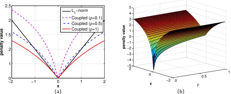
Theorem 3 In the special case where f(γi) =b, then
gVB(xi, ρ)≡
2|xi|
|xi|+ q
x2 i + 4ρ
+ log
2ρ+x2i +|xi| q
x2i + 4ρ
. (14)
Figures 1 (a) and (b) display 1D and 2D plots of this penalty function. It is worth spending some time here to examine this particular selection for f (and therefore gVB) in
detail since it elucidates many of the mechanisms whereby VB, with all of its attendant approximations and heuristics, can affect improvement over MAP regardless of the true noise level.
In the limit asρ→0, the first term in (14) converges to the indicator functionI[xi6= 0], and thus when we sum over i we obtain the `0 norm of x, which represents a canonical measure of sparsity, or a count of the nonzero elements in a vector.7 The second term in (14), when we again sum over i, converges to P
ilog|xi|, ignoring a constant factor. Sometimes referred to as Gaussian entropy, this term can also be connected to the`0 norm via the relations kxk0 ≡ limp→0Pi|xi|p and limp→0 1pPi(|xi|p −1) = Pilog|xi| (Wipf et al., 2011). Thus the cumulative effect whenρbecomes small is an image prior that closely mimics the highly non-convex (in|xi|)`0 norm which favors maximally sparse solutions. In contrast, when ρ becomes large, it can be shown that both terms in (14), when combined for all i, approach scaled versions of the convex `1 norm. Additionally, this scaling turns out to be principled in the sense described in Wipf and Wu (2012); Zhang and Wipf (2013). For intermediate values ofρ between these two extremes, we obtain agVBthat becomes less concave with respect to each|xi|asρincreases in the formal sense of relative concavity discussed in Section 3.1. In particular, we have the following:
6. The Jeffreys prior is of the formp(x)∝1/|x|, which represents an improper distribution that does not
integrate to one.
−20 −1 0 1 2 1
2 1.5 2 2.5
x
penalty value
L 1−norm Coupled (ρ=0.1) Coupled (ρ=0.5) Coupled (ρ=1)
(a)
0
0.5
1
−2 0 2 −5 −4 −3 −2 −1 0 1 2 3 4 5
ρ
x
penalty value
(b)
Figure 1: (a) A 1D example of the coupled penaltygVB(x, ρ) (normalized) with different ρ
values assumingf is a constant. The `1 norm is included for comparison. (b) A 2D example surface plot of the coupled penalty functiongVB(x, ρ);f is a constant.
Corollary 4 If f(γi) =b, then gVBρ1 ≺g ρ2
VB for ρ1 < ρ2.
Thus, as the noise level λis increased, ρ increases and we have a penalty that behaves more like a convex (less sparse) function, and so becomes less prone to local minima. In contrast, askk¯k2
2 is increased, meaning thatρis now reduced, the penalty actually becomes
more concave with respect to |xi|. This phenomena is in some ways similar to certain homotopy continuation sparse estimation schemes (e.g., Chartrand and Yin 2008), where heuristic hyperparameters are introduced to gradually introduce greater non-convexity into canonical compressive sensing problems, but without any dependence on the noise or other factors. The key difference here with VB however is that penalty shape modulation is explicitly dictated by both the noise levelλand the kernel kin an integrated fashion. 8
To summarize then, the ratioρ can be viewed as modulating a smooth transition of the penalty function shape from something akin to the non-convex`0 norm to a properly-scaled
`1 norm. In contrast, conventional MAP-based penalties onxare independent fromkorλ, and thus retain a fixed shape. The crucial ramifications of this coupling and ρ-controlled shape modification/augmentation exclusive to the VB framework will be addressed in the following two subsections. Other choices for f, which exhibit a partially muted form of this coupling, will be considered in Section 3.7, which will also address a desirable form of invariance that only exists when f is a constant.
3.4 Noise Dependency Analysis
The success of practical VB blind deconvolution algorithms is heavily dependent on some form of stagewise coarse-to-fine approach, whereby the kernel is repeatedly re-estimated at
successively higher resolutions. At each stage, a lower resolution version is used to initial-ize the estimate at the next higher resolution. One way to implement this approach is to initially use large values of λ(regardless of the true noise level) such that only dominant, primarily low-frequency image structures dictate the optimization (Levin et al., 2009). Dur-ing subsequent iterations as the blur kernel begins to reflect the correct coarse shape,λcan be gradually reduced to allow the recovery of more detailed, fine structures.
A highly sparse (concave) prior can ultimately be more effective in differentiating sharp images and fine structures than a convex one. Detailed supported evidence for this claim can be found in Fergus et al. (2006); Levin et al. (2007); Krishnan and Fergus (2009); Cho et al. (2012), as well as in Section 4 below. However, if such a prior is applied at the initial stages of estimation, the iterations are likely to become trapped at suboptimal local minima, of which there will always be a combinatorial number. Moreover, in the early stages, the effective noise level is actually high due to errors contained in the estimated blur kernel, and exceedingly sparse image penalties are likely to produce unstable solutions.
Given the reformulation outlined above, we can now argue that VB implicitly avoids these problems by beginning with a largeλ(and therefore a largeρ), such that the penalty function is initially nearly convex in |xi|(see Figure 1). In this situation, the data fidelity term λ1ky−k∗xk22 from (12) is de-emphasized because of the inverse dependency on λ, and small edges and structures will be ignored. Hence an approximately convex penalty is generally sufficient for resolving the remaining strong edges. As the iterations proceed and fine structures need to be resolved, the penalty function is made less convex (more concave) as λis reduced, but the risk of local minima and instability is ameliorated by the fact that we are likely to be already in the neighborhood of a desirable basin of attraction. Additionally, the implicit noise level (or modeling error) is now substantially lower.
This kind of automatic ‘resolution’ adaptive penalty shaping is arguably superior to conventional MAP approaches based on (3), where the concavity/shape of the induced sep-arable penalty function is kept fixed regardless of the variation in the noise level or scale, i.e., at different resolutions across the coarse-to-fine hierarchy. In general, it would seem very unreasonable that the same penalty shape would be optimal across vastly different noise scales. This advantage over MAP can be easily illustrated by simple head-to-head comparisons where the underlying prior distributions are identical; Section 3.6 below con-tains one such example. Additionally, this phenomena can be significantly enhanced by automatically learning λas discussed in Section 5.
3.5 Blur Dependency Analysis
There are many different viewpoints for understanding how the blur dependency of the VB penalty gVB contributes to successful deblurring results. Here we consider potentially one
of the most transparent.
Because the blur kernel appears judiciously in all three terms in (12), with a slight repa-rameterization and subsequent algebraic manipulation, we may consolidate terms leading to the equivalent revised formulation of (12) given by
L(˜x,k)˜ , 1 λ
y−k˜∗x˜ 2 2+
X i
where ˜xi,xikk¯k2 for alliand, with slight abuse of notation, ˜kdenotes a normalized kernel such that the resulting convolution matrix Hhas columns of unit norm. In other words, if x∗ and k∗ represent the optimal solution to (12), then ˜x∗ = x∗kk¯∗k2 and ˜k∗ =k∗/kk¯∗k2 are the optimal solution to (15), at least whengVBis given by (14). Hence we see that, once
the kernel operator is constrained to have unit`2 norm,no additional kernel penalization is
included whatsoever. Consequently then, to the extent VB is successful, we observe that an additional kernel penalty, and any associated tuning parameter, is completely unnecessary. Additionally, with the kernel fixed, solving for ˜x now represents a standardized sparse estimation problem, with a quadratic data-fit term now characterized by a design matrix Hwith consistent `2 normalized columns.
Note that essentially all previous blind deblurring algorithms assume what amounts to an `1 normalized kernel satisfying Piki = 1 (since each element of the sum must be positive, the corresponding convolution matrix H will have`1 normalized columns except at the boundary). But in the context of a quadratic data fit term as used by deblurring algorithms, this is unlikely to be optimal as it will apply some implicit pressure on the estimated kernel towards the no-blur solution (k = δ), potentially counteracting, at least in part, the push for sparse image estimates. This occurs because kernels near the delta solution will increase the `2 column norms of H when the `1 norm is fixed, which then allows for relatively smaller image coefficients x by virtue of the quadratic data term. These smaller coefficients then reduce any non-decreasing penalty on the magnitudes of x, reducing the overall cost function. Additionally, in much more complex non-uniform deblurring environments, this undesirable effect is considerably more pronounced (Zhang and Wipf, 2013).
In the context of VB however, this `1 normalization is implicitly switched to `2 normal-ization via the mechanism outlined above leading to (15), and hence it is entirely inconse-quential to VB. In contrast, MAP has no such agency, and therefore it is not surprising that the majority of MAP algorithms explicitly include an additional `2 kernel penalty which helps to counteract movement towards no-blur solutions. The disadvantage of course is that an additional image-dependent tuning parameter is required as well to balance the resulting contribution. We could, however, alternatively consider replacing the `1 norm constraint in MAP with `2-norm constraints as in (15), although this complicates the optimization process considerably, whereas VB handles this automatically.9
3.6 Illustrative Example using 1D Signals
Here we will briefly illustrate some of the distinctions between MAP and VB discussed thus far where other confounding factors have been conveniently removed. For this purpose we consider a simplified noiseless situation where the optimal λvalue is zero, and we consider the image prior produced whenf(γ) =bas introduced in Section 3.3 (later Section 3.7 will
9. One potential way around these complications for MAP would be to replace the non-convex constraint
kk¯˜k2 = 1 with the convex quadratic onekk¯˜k2 ≤1, ignoring boundary effects which would complicate
things dramatically by requiringmadditional constraints, one for each element ofx. While in uniform
blur models this could be effective since the optimal solution should satisfy kk¯˜k2 = 1 anyway, in
argue that this selection is in some sense optimal). For MAP we also include the kernel penalty mlogkk¯k2
2 from (12) which will facilitate more direct comparisons with VB below. Given these assumptions, the associated MAP problem from (3) is easily shown to be
min
x,k
1
λky−k∗xk
2 2+
X i
2 log|xi|+ 2mlogk¯kk2, (16)
where the image penalty is obtained by applying a−2 log transformation to (11) giving
−2 log
max
γi≥0N(xi; 0, γi)
≡2 log|xi|. (17)
Irrelevant additive constants have been excluded. Conveniently, since
X i
2 log|xi|+ 2mlogkk¯k2 = X
i
2 log |xi| kk¯k2
, (18)
we can reparameterize (16) using ˜x such that the kernel penalty is removed and the con-straintkk˜¯k2 = 1 is enforced just as with VB. Consequently, in the limit asλ→0, based on the equivalency derived from Corollary 1, both VB and MAP are then effectively solving
min ˜
x,˜k
X i
log|x˜i|, s.t. y= ˜k∗x˜, kk˜¯k2 = 1. (19)
Moreover, given the arguments made in Section 3.3, the penalty on ˜xis more or less equiv-alent to the `0 norm up to inconsequential scaling and translations. Thus, (19) effectively reduces to
min ˜
x,k˜
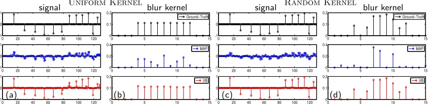
kx˜k0, s.t. y= ˜k∗x˜, k˜¯kk2= 1. (20) Therefore at this simplified, stripped-down level both VB and MAP are merely minimizing the`0norm ofxsubject to the linear convolutional constraint. Of course we do not attempt to solve (20) directly, which is a difficult combinatorial problem in nature. Instead for both VB and MAP we begin with a large λ and gradually reduce it towards zero as part of a multi-resolution approach designed to avoid bad local minima as described in Section 3.4. For this reduction schedule of λwe use β = 1.15 in Algorithm 1 (this value is taken from Levin et al. 2011a).10 While equivalent when λ → 0, before λ becomes small the VB and MAP cost functions will behave very differently, leading to a radically different optimization trajectory terminating at different locally minimizing solutions to (20).
The superiority of the VB convergence path will now be demonstrated with a synthetic 1D signal composed of multiple spikes. This signal is convolved with two different blur kernels, one uniform and one random, creating two different blurry observations. Refer to Figure 2 (first row) for the ground-truth spike signal and associated blur kernels. We then apply the MAP and VB blind deconvolution algorithms, with the same prior (f equals a constant) andλreduction schedule, to the blurry test signals and compare the quality of the
10. The corresponding MAP algorithm can be implemented by simply setting C to zero before the q(γi)
update in Algorithm 1, with guaranteed convergence to some local minima. For both MAP and VB, the
reconstructed blur kernels and signals. The recovery results are shown in Figure 2 (second and third rows), where it is readily apparent that VB produces superior estimation quality of both kernel and image. Additionally, the signal recovered by VB is considerably sparser than MAP, indicating that it has done a better job of optimizing (20), consistent with our previous analysis. This is not to say that MAP cannot potentially be effective with careful tuning and initialization (perhaps coupled with additional regularization factors or clever optimization schemes), only that VB is much more robust in its present form.
Note that this demonstrable advantage of VB is entirely based on an improved con-vergence path, since VB and MAP possess an identical constellation of local minima once
λ= 0. Moreover, it is unrelated to any putative advantage of solving (4) over (3). We will revisit this latter point in Section 4.
0 20 40 60 80 100 120 −1
0 1
0 20 40 60 80 100 120 −1
0 1
0 20 40 60 80 100 120 −1
0 1
(a)
signal Uniform Kernel
0 5 10 15
0 0.1 0.2
Ground−Truth
0 5 10 15
0 0.2 0.4
MAP
0 5 10 15
0 0.1 0.2 VB (b) blur kernel
0 20 40 60 80 100 120 −1
0 1
0 20 40 60 80 100 120 −1
0 1
0 20 40 60 80 100 120 −1
0 1
signal Random Kernel
(c)
0 5 10 15
0 0.1 0.2
Ground−Truth
0 5 10 15
0 0.2 0.4
MAP
0 5 10 15
0 0.1 0.2 VB blur kernel (d)
Figure 2: 1D deblurring example using MAP and VB approaches assuming the same under-lying image priorp(x). (a)-(b) results with a uniform blur kernel; (c)-(d) results with a random blur kernel.
3.7 Other Choices for f
Because essentially any sparse prior onxcan be expressed using the alternative variational form from (11), choosing such a prior is tantamount to choosing f which then determines
gVB. Theorem 2 suggests that a concave, non-decreasing f is useful for favoring sparsity
(assumed to be in the gradient domain). Moreover, Theorem 3 and subsequent analyses suggest that the simplifying choice where f(γ) = b possesses several attractive properties regarding the relative concavity of the resulting gVB. But what about other selections forf
and therefore gVB?
While directly working with gVB can sometimes be limiting (except in certain special
cases like f(γ) =b from before), the variational form of (13) allows us to closely examine the relative concavity of a useful proxy. Let
ψ(γi, ρ),log(ρ+γi) +f(γi). (21)
Then for fixedλand k the VB estimation problem can equivalently be viewed as solving
min
x,γ≥0 1
λky−k∗xk
2 2+
X i
x2i γi
+ψ(γi, ρ)
It now becomes clear that the sparsity of xand γ are intimated related. More concretely, assumingf is concave and non-decreasing (as motivated by Theorems 2 and 3), then there is actually a one-to-one correspondence in that wheneverxi = 0, the optimalγi equals zero as well, and vice versa.11 Therefore we may instead examine the relative concavity ofψfor different ρ values, which will directly determine the sparsity ofγ and in turn, the sparsity of x. This then motivates the following result:
Theorem 4 Let ρ1 < ρ2 and assume that f satisfies the conditions of Theorem 2. Then
ψρ1 ≺ψρ2 if and only if f(γ) =aγ+b, witha≥0.
Thus, although we have not been able to formally establish a relative concavity result for all general gVB directly, Theorem 4 provides a nearly identical analog allowing us to
draw similar conclusions to those detailed in Sections 3.4 and 3.5 whenever a general affine
f is adopted. Perhaps more importantly, it also suggests that as f deviates from an affine function, we may begin to lose some of the desirable effects regarding the described penalty shape modulation.
While previously we closely scrutinized the special affine case where f(γ) = b, it still remains to examine the more general affine form f(γ) = aγ+b, a > 0. In fact, it is not difficult to show that asais increased, the resulting penalty on xincreasingly resembles an
`1norm with lesser dependency onρ, thus severely muting the effect of the shape modulation that appears to be so effective (see arguments above and empirical results section below). So there currently does not seem to be any advantage to choosing some a >0 and we are left, out of the multitude of potential image priors, with the conveniently simple choice of f(γ) = b, where the value of b is inconsequential. Experimental results support this conclusion: namely, asais increased from zero performance gradually degrades (results not shown for space considerations).
As a final justification for simply choosing f(γ) =b, there is a desirable form of invari-ance that uniquely accompanies this selection.
Theorem 5 If x∗ and k∗ represent the optimal solution to (12) under the constraint
P
iki= 1, thenα−1x∗ andαk∗ will always represent the optimal solution under the modified constraint P
iki=α if and only iff(γ) =b. Additionally, minimizing (12) is equivalent to minimizing (15) if and only iff(γ) =b.
This is unlike the myriad of MAP estimation techniques or VB with other choices of
f, where the exact calibration of the constraint can fundamentally alter the form of the optimal solution beyond a mere rescaling. Moreover, if such a constraint on k is omitted altogether, these other methods must then carefully tune associated trade-off parameters, so in one way or another this lack of invariance will require additional tuning.
Interestingly, Babacan et al. (2012) experiments with a variety of VB algorithms using different underlying image priors, and empirically find that f as a constant works best;
11. To see this first consider xi = 0. The x2i/γi term can be ignored and so the optimal γi need only
minimize log(ρ+γi) +f(γi), which is concave and non-decreasing wheneverf is. Therefore the optimal
γi is trivially zero. Conversely ifγi= 0, then there is effectively an infinite penalty on xi, and so the
however, no rigorous explanation is given for why this should be the case.12 Thus, our results provide a powerful theoretical confirmation of this selection, along with a number of useful attendant intuitions.
3.8 Analysis Summary
To summarize this section, we have shown that the shape of the effective VB image penalty is explicitly controlled by the ratio of the noise variance to the squared kernel norm, and that in many circumstances this leads to a desired mechanism for controlling relative concavity and balancing sparsity, largely mitigating issues such as local minima that compromise the convergence of more traditional MAP estimators. We have then demonstrated a unique choice for the image prior (i.e., when f is constant) such that this mechanism is in some sense optimal and scale-invariant. Of course we readily concede that different choices for the image prior could still be useful when other factors are taken in to account. We also emphasize that none of this is meant to suggest that real imaging data follows a Jeffreys prior distribution (which is produced when f is constant). We will return to this topic in Section 4 below. Overall, this perspective provides a much clearer picture of how VB is able to operate effectively and how we might expect to optimize performance.
While space precludes a detailed treatment, many natural extensions to VB are sug-gested by these developments. For example, in the original formation of VB given by (7) it is not clear the best way to incorporate alternative noise models because the required inte-grations are no longer tractable. However, when viewed alternatively using (12) it becomes obvious that different data-fidelity terms can easily be substituted in place of the quadratic likelihood factor. Likewise, given additional prior knowledge about the blur kernel, there is no difficulty in substituting for the`2-norm onk or the uniform convolutional observation model to reflect additional domain knowledge. Thus, the proposed reformulation allows VB to inherit most of the transparent extensibility previously reserved for MAP.
We may also consider these ideas in the context of existing MAP algorithms, which adopt various structure selection heuristics, implicitly or explicitly, to achieve satisfactory performance (Shan et al., 2008; Cho and Lee, 2009; Xu and Jia, 2010). This can be viewed as adding additional image penalty terms and trade-off parameters to (3). For example, Shan et al. (2008) incorporates an extra local penalty on the latent image, such that the gradients of small-scale structures in the recovered image are close to those in the blurry image. Thus they will actually contribute less to the subsequent kernel estimation step, allowing larger structures to be captured first. Similarly, a bilateral filtering step is used for pruning out small scale structures in Cho and Lee (2009). Finally, Xu and Jia (2010) develop an empirical structure selection metric designed such that small scale structures can be pruned away by thresholding the corresponding response map, allowing subsequent kernel estimation to be dominated by only large-scale structures.
12. Based on a strong simplifying assumption that the covarianceCfrom Algorithm 1 is a constant, Babacan
et al. (2012) provides some preliminary discussion regarding possibly why VB may be advantageous over
MAP. However, when C is constant, the analysis easily reduces to a standard penalized regression
problem, and hence this material can already be found in the sparse estimation literature (e.g., see Palmer et al. 2006; Wipf et al. 2011 and related references). Our key contribution is to explicitly account
Generally speaking, existing MAP strategies face a trade-off: either they must adopt a highly sparse image prior needed for properly resolving fine structures (see Section 4) and then deal with the attendant constellation of problematic local minima,13 or rely on a more smooth image prior augmented with compensatory structure-selection measures such as those described above to avoid bad global solutions. In contrast, we may interpret the coupled penalty function intrinsic to VB as a principled alternative with a transparent, in-tegrated functionality for estimation at different resolutions without any additional penalty factors, trade-off parameters, or complexity.
4. Maximal Sparsity vs. Natural Image Statistics
Levin et al. (2009, 2011a,b), which represents the initial inspiration for our work, presents a compelling and highly influential case that joint MAP estimation overx andk generally favors a degenerate, no-blur solution, meaning that k will be a delta function, even when the assumed image priorp(x) reflects the true underlying distribution ofx, meaningp(x) =
ptrue(x), and p(k) is assumed flat in the feasible region.14 In turn, this is presented as a primary argument for why MAP is inferior to VB. As this line of reasoning is considerably different from that given in Section 3, here we will take a closer look at these orthogonal perspectives in the hopes of providing a clarifying resolution.
To begin, it helps to revisit the formal analysis of MAP failure from Levin et al. (2011b), where the following specialized scenario is presented. Assume that a blurry image y is generated byy=k∗∗x∗, where kk∗k2 1 and each true sharp image gradientx∗i is drawn iid from the generalized Gaussian distribution ptrue(x∗i) ∼ exp(−|x∗i|p), 0 < p ≤ 1. Now consider the minimization problem
min
x,k
X i
|xi|p s.t. y=k∗x. (23)
Solving (23) is equivalent to MAP estimation over x and k under the true image prior
ptrue(x) and an implicitly assumed flat prior on k within the previously specified kernel constraint set. In the limit as the image grows arbitrarily large, (Levin et al., 2011b, Claim 2) proves that the no-blur delta solution{x=y,k=δ}will be favored over the true solution {x=x∗,k=k∗}. Intuitively, this occurs because the blurring operator kcontributes two opposing effects:
1. It reduces a measure of the imagesparsity, which increasesP
i|yi|p, and 2. It broadly reduces the overall imagevariance, which reducesP
i|yi|p.
Depending on the relative contributions, we may have the situation where the second effect dominates such that P
i|yi|p may be less than P
i|x
∗
i|p, meaning the cost function value
13. Appropriate use of continuation methods such as the algorithm from Chartrand and Yin (2008) may help in this regard.
14. Note that Levinet al. frequently use MAPx,kto refer to joint MAP estimation over bothkandx(Type
I) while using MAPkfor MAP estimation ofkalone afterxhas been marginalized out (Type II). In this
terminology, MAPk then represents the inference ideal that VB purports to approximate, equivalent to
at the blurred image is actually lower than at the true, sharp image. Consequently, MAP estimation may not be reliable.
Our conclusions then suggest a sort of paradox: in Section 3 we have argued that VB is actually equivalent to an unconventional form of MAP estimation over x, but with an intrinsic mechanism for avoiding bad local minima, increasing the chances that a good global or near-global minima can be found. Moreover, at least in the noiseless case (λ→0), any such minima will be exactly equivalent to the standard MAP solution by virtue of Corollary 1. However, based on the noiseless analysis from Levin et al. above, any global MAP solution is unlikely to involve the true sharp image when the true image statistics are used for p(x), meaning that VB performance should be poor as well even at a global solution. Thus how can we reconcile the positive performance of VB actually observed in practice, and avoidance of degenerate no-blur solutions, with Levinet al.’s characterization of the MAP cost function?
First, when analyzing MAP, Levin et al. consider only a flat prior on k within the constraint set P
iki = 1 and ki ≥ 0. However, MAP estimation may still avoid no-blur solutions when equipped with an appropriate non-flat kernel prior and associated trade-off parameter. Likewise under certain conditions described in Section 3.5, VB naturally substitutes in a quadratic normalization constraint forkthat we have argued disfavors no-blur solutions automatically. Moreover, VB introduces this normalization in a convenient form devoid of additional tuning parameters.
Secondly, the argument in Levin et al. breaks down when the true sharp image x∗ is actually sparse in the canonical sense, meaning the distribution of each element includes a delta function at zero, i.e.,
ptrue(x∗i) =αδ(xi∗) + (1−α)ρ(xi), (24) whereρ is an arbitrary distribution and α∈[0,1] is a constant. Clearly samples from (24) will include some elements exactly equal to zero with probability at least α.
Lemma 1 Let x∗ be distributed iid with elements drawn from (24) and let y = k∗ ∗x∗
for some non-negative kernel k∗. Then with probability approaching one as the image size grows large
k∗,x∗ = arg min
k,x:y=k∗xlogptrue(x
∗
i) = arg min
k,x:y=k∗xkxk0. (25)
The proof is straightforward and we do not reproduce it here. Regardless, this result demonstrates that exactly sparse images can in fact be recovered using MAP or equivalently the`0 norm, the latter of which is actually blind to the distribution of non-zero coefficients
ρ(xi). Intuitively, this occurs because these measures are entirely immune to changes in variance and only sensitive to sparsity; hence any blurring operation will only increase either penalty function in the feasible region. So immediately we may conclude that, assuming we have some way of solving (25), we should not discount MAP or`0 minimization as a viable means for recovering sparse images. And importantly, the exact distribution of nonzero coefficients is irrelevant as long as some degree of sparsity exists.
hold and MAP estimation seems to have been discredited. However, we would argue that MAP can still be salvaged if we are willing to intentionally allow mismatch between the true image prior and the image prior which forms the basis of our MAP estimator. More specifically, we suggest replacing the true image statisticsptruewith the`0 norm. However, solving (25) directly will obviously not be effective when there are no exactly zero-valued coefficients.
Fortunately there is a simple way around this. In the regime wheren≈m, meaning the sharp and blurry images yand x are large relative to the size of kand therefore of nearly equal dimension, the generalized Gaussian distribution withp≈[0.5,0.8] is a compressible distribution in the sense described in Cevher (2009). In words, this means that the sorted magnitudes of samples from this distribution exhibit a power-law decay and hence can be well-approximated by sparse signals. Consequently, there will exist some sparse ˆx with kxˆk0 m such that ky−k∗ ∗xˆk2
2 < for some small . In contrast, each element of the blurry image y is a summation of many elements of x∗ via the blur operation, and therefore, by central limit theorem arguments each element, while not exactly iid, will approach samples from a Gaussian distribution (exactly so for large enough blur kernels), which is not a compressible distribution. Therefore, if we solve a relaxed version of (25) given by
min
x,k kxk0, s.t. ky−k∗xk
2
2 < , (26)
with an appropriate choice for , then we are very likely to obtain the true blur kernelk∗, and a close sparse approximation to x∗. Conversely it is very unlikely that the solution will be x =y and k =δ. Therefore, just because x∗ may not be exactly sparse, we may nonetheless locate a sparse approximation ˆx that is sufficiently reasonable such that the unknownk∗ can still be estimated accurately, facilitating a later non-blind, image domain estimation step.
Overall then, the success of the `0 norm penalty in the context of MAP estimation speaks to the following point: it is more important that the assumed image prior p(x) = exp[−12gx(x)] be maximally discriminative with respect to blurred and sharp images, as
opposed to accurately reflecting the statistics of real images. Mathematically, this implies that it is much more important that we have p(k∗x∗) p(ˆx) for some ˆx such that k∗x∗ ≈k∗x, than we enforceˆ p(x) = ptrue(x), even if ptrue(x) were known exactly. This is because the sparsity/variance trade-off described above implies that it may often be the case thatptrue(k∗x∗)> ptrue(ˆx) leading to the no-blur solution.
Obviously from a practical standpoint solving (26) represents a difficult, combinatorial optimization problem with numerous local minima. However, to the extent that the VB image penaltygVBapproximates the`0norm, the VB cost (12) can be viewed as an approx-imate Lagrangian form of (26), but augmented with an adaptive shape modulation that helps to circumvent these local minima. Thus we can briefly summarize largely why VB can be superior to MAP: VB allows us to use a near-optimal image penalty, one that is maximally discriminative between blurry and sharp images, but with a reduced risk of get-ting stuck in bad local minima during the optimization process. Overall, these conclusions provide a more complete picture of the essential differences between MAP and VB.
Levin et al. (2011b) prove that whenp(x) =ptrue(x), then in the limit as the image grows large the MAP estimate fork, after marginalizing overx (Type II), will equal the truek∗. But there is no inherent contradiction with our results, since it should now be readily appar-ent that VB is fundamappar-entally differappar-ent than solving minkp(k|y), and therefore justification
for the latter cannot be directly transferred to justification for the former. This highlights the importance of properly differentiating various forms of Bayesian inference, both in the context of blind image deblurring and beyond to widespread application domains.
Natural image statistics are ideal in cases where y and x grow large and we are able to integrate out the unknown x, benefiting from central limit arguments when estimating k alone. However, when we jointly compute MAP estimates of both x and k (Type I) as in (3), we enjoy no such asymptotic welfare since the number of unknowns increases proportionally with the sample size. One of the insights of our paper is to show that, at least in this regard, VB is on an exactly equal footing with Type I MAP, and thus we must look for theoretical VB justification elsewhere, leading to the analysis of relative concavity, local minima, invariance, maximal sparsity, etc. presented herein.
5. Learning λ
While existing VB blind deconvolution algorithms typically utilize some pre-assigned de-creasing sequence forλas described in Section 3.4 and noted in Algorithm 1, it is preferable to have λlearned automatically from the data itself as is common in other applications of VB. In the case of blind deblurring, we expect that such a learned λ, with an image-dependent trajectory, may better modulate the penalty curvature discussed in Section 3.4. In contrast, a fixed, pre-defined decreasing sequence is likely to be miscalibrated as it will not reflect the current quality of image and kernel estimates during each iteration. Addi-tionally, the alternative strategy of learning λ has the conceptual appeal of an integrated cost function that is universally reduced even as λ is updated, unlike Algorithm 1 where theλreduction step may in fact increase the overall cost.
However, current VB deblurring papers either do not mention such a seemingly obvious alternative (perhaps suggesting that the authors unsuccessfully tried such an approach) or explicitly mention that learning λ is problematic but without concrete details. For example, Levin et al. (2011b) observed that the noise level learning used in Fergus et al. (2006) represents a source of problems as the optimization diverges when the estimated noise level decreases too much. But there is no mention of whyλmight decrease too much, and further details or analyses are absent.
Interestingly, the perspective presented herein provides some direct insights into howλ
may be effectively learned. Consider minimization of the revised VB cost function (12) over x,k, and now λas well. Because x∈Rm and y∈
Rn withm > n, for a fixedk there are
A problem then arises because it can be shown that gVB(0, ρ) → −∞ as ρ → 0 for all
non-decreasingf.15 Consequently, we can always trivially drive the VB cost function (12) to−∞ using any basic feasible solution combined with λ→ 0, regardless of the quality of the solution. Now because of the disparity in dimensionality mentioned above, there will always be feasible solutions to y =k∗xwith at least m−n or more elements of x equal to zero. Thus, at any one of these solutions the VB cost function (12) can then be driven to −∞ with λ → 0. Unless the true x actually has many exactly zero-valued elements, this will represent a globally degenerate minimizing solution for a broad class of f. And even for other choices forf, a slightly more subdued form of this same degeneracy will still exist since the VB-specific regularization fundamentally favors λ being small: essentially the log(γi+ρ) factor in (13) will always favor ρ, and therefore λ being small. The 1/λ weighting of ky−k∗xk22 is not sufficient for counteracting this effect given the multitude of feasible solutions such thaty=k∗x.
And even for other choices for f, a slightly more subdued form of this same degeneracy will still persist since the existing VB-specific regularization fundamentally favors λbeing small: essentially the log(γi+ρ) factor in (13) will always favor ρ, and therefore λbeing small. The 1/λweighting ofky−k∗xk22 is not sufficient for counteracting this effect given the multitude of feasible solutions such thaty=k∗x.
However, these degeneracies can be circumvented with an additional penalty factor on
λ that is naturally motivated by this framework. Specifically, we propose to append the penalty function
v(λ) = (n−m) logλ+ d
λ (27)
to (12), wheredis assumed to be a small positive constant. The first term in (27) directly counteracts the degeneracy of basic feasible solutions by providing an equal and opposite barrier to arbitrary solutions with λ → 0 and kxk0 = m−n. Additionally, when f is a constant as we have argued previously represents a well-motivated selection, then it can be shown that this additional penalty represents a very principled approximation to what the true λ penalty should be if the original VB formulation from (6) were not factorized as in (7). Additionally, for other choices of f, (12) can be similarly modified to provide a consistent estimator forλin the sense described in Wipf and Wu (2012).
As justification for the second term in (27), note that this added factor is proportional to 1/λky−k∗xk22, but acts as an interpretable barrier preventingλfrom ever going below
d/n, which remains a possibility even with the (n−m) logλ term in place. In fact it is easily shown (see Appendix B) that any λ minimizing the cost function (12) augmented with the penaltyv(λ) must satisfyλ≥d/n, which can be viewed as a lower-bound on what 1/nky−k∗xk22 should be.16
In practice, we have found the fixed value d=n×10−4 to be highly effective across a wide range of images and testing scenarios, including all reported results in Section 6 and
15. Based on (13), it is clear that the optimizingγi value for computing gVB(0, ρ) will be γi = 0. When
ρ→0, we then have log(γi+ρ)→ −∞, and thereforegVB(0, ρ)→ −∞. Graphically, Figure 1 (b) also
reveals this effect, showing that if we were to jointly minimize over both xand ρ, the{0,0}solution is
heavily favored.
16. While it could be argued that settingd to a larger value could obviate the need for the (n−m) logλ
penalty altogether, we would lose considerable interpretability, connection with the original VB problem,