The Thirty-Third AAAI Conference on Artificial Intelligence (AAAI-19)
Point Cloud Processing via Recurrent Set Encoding
Pengxiang Wu,
1Chao Chen,
2Jingru Yi,
1Dimitris Metaxas
11Department of Computer Science, Rutgers University, NJ, USA,{pw241, jy486, dnm}@cs.rutgers.edu 2Department of Biomedical Informatics, Stony Brook University, NY, USA, [email protected]
Abstract
We present a new permutation-invariant network for 3D point cloud processing. Our network is composed of a recurrent set encoder and a convolutional feature aggregator. Given an unordered point set, the encoder firstly partitions its ambi-ent space into parallel beams. Points within each beam are then modeled as a sequence and encoded into subregional ge-ometric features by a shared recurrent neural network (RNN). The spatial layout of the beams is regular, and this allows the beam features to be further fed into an efficient 2D convolu-tional neural network (CNN) for hierarchical feature aggrega-tion. Our network is effective at spatial feature learning, and competes favorably with the state-of-the-arts (SOTAs) on a number of benchmarks. Meanwhile, it is significantly more efficient compared to the SOTAs.
Introduction
Point cloud is a simple and compact geometric representa-tion of 3D objects, and has been broadly used as the stan-dard output of various sensors. In recent years, the analysis of point clouds has gained much attention due to its wide ap-plication in real world problems such as autonomous driving (Chen et al. 2017), robotics (Kehoe et al. 2015), and naviga-tion (Liu 2016). However, it is nontrivial to solve such tasks using traditional deep learning tools, e.g., convolutional neu-ral networks (CNNs). Unlike a 2D image with regularly packed pixels, a point cloud consists of sparse points with-out a canonical order. Moreover, the spatial distribution of a point cloud is heterogeneous due to factors in data acquisi-tion, e.g., perspective effects and radial density variations.
Due to the 3D nature of the problem, various methods have been proposed to convert a point cloud into a 3D vol-umetric representation, to which 3D CNNs are then applied (Wu et al. 2015; Maturana and Scherer 2015b). However, despite their success in analyzing 2D images, CNNs are not satisfactory in this context. The commonly used 3D CNN is extremely memory consuming, and thus can not be trained efficiently. A more serious issue is that converting a point cloud into a volumetric representation introduces quantiza-tion artifacts and loses fine-scale geometric details.
Better performance has been achieved by deep networks that avoid the volumetric convolutional architechture and
Copyright c2019, Association for the Advancement of Artificial Intelligence (www.aaai.org). All rights reserved.
operate directly on point clouds. Representative works in-clude PointNet (Qi et al. 2017a) and PointNet++ (Qi et al. 2017b), which process point clouds by combining multi-layer perceptron (MLP) network with symmetric operations (e.g., max-pooling) to learn point features globally or hierar-chically. Inspired by PointNet, several recent methods have been proposed to further improve the point feature represen-tation (Shen et al. 2018; Xie et al. 2018; Li, Chen, and Lee 2018). This class of networks are invariant to input permuta-tion and have achieved state-of-the-art results. However, due to the reliance on the coarse feature pooling technique, they fail to fully exploit fine-scale geometric details.
In this work, we aim to completely bypass the coarse pooling-based technique, and propose a new deep network for point cloud data. At the core of our method is arecurrent set encoder, which divides the ambient domain into parallel
beams and encodes the points within each beam as subre-gional geometric features with an RNN. Our key observa-tion is that when the beam is of moderate size, the RNN is approximately dealing with a sequence of points, as a beam only contains points near a 1D line. Such a sequential in-put largely benefits the learning of RNN. Meanwhile, notic-ing that the beams are packed in a regular spatial layout, we use a 2D CNN to further analyze the beam features (called the convolutional feature aggregator). Being efficient and powerful at feature learning, the 2D CNN can effectively aggregate the subregional features into a global one, while further benefiting the RNN learning in return. Our method (see Fig. 1) is surprisingly efficient and effective for point cloud processing. It is invariant to point order permutation, and competes favorably with the state-of-the-arts (SOTAs) in terms of both accuracy and computational efficiency.
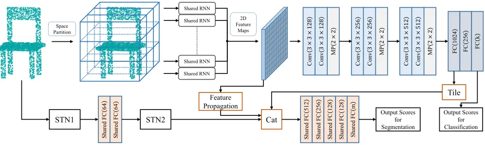
Shared RNN Shared RNN Shared RNN Shared RNN Space Partition 2D Feature Maps Conv 3 × 3 × 128 MP 2 × 2 Conv 3 × 3 × 128 Conv 3 × 3 × 256 MP 2 × 2 Conv 3 × 3 × 256 Conv 3 × 3 × 512 MP 2 × 2 Conv 3 × 3 × 512 FC 1024 FC 256 FC k Output Scores for Classification STN1 Sh ar ed FC 64 Sh ar ed FC 64 STN2 Tile Cat Sh ar ed FC 512 Sh ar ed FC 256 Sh ar ed FC 128 Sh ar ed FC 128 Sh ar ed FC m Output Scores for Segmentation Feature Propagation
Figure 1: The architecture of RCNet. In the recurrent set encoder, the ambient space of input points is partitioned into parallel beams, where the enclosed points are encoded by a shared RNN. The subregional features from each beam are later processed by a 2D CNN. Depending on the tasks, the aggregated global features are fed forward directly for shape prediction, or tiled and concatenated with the per-point features for semantic segmentation. The feature propagation refers to the operation that propagates the non-local features within each beam to the corresponding component points. The other operations used are: Conv (2D convolution), MP (2D max-pooling), FC (fully connected layer). Batchnorm and ReLU are used in all layers except the last one, and the shared FC is applied per point. Numbers in parentheses represent the size of operation, and the hidden size of RNN is 64 and 128 for classification and segmentation tasks, respectively. The STN block refers to the spatial transformer network (Jaderberg et al. 2015; Qi et al. 2017a). It outputs a transformation matrix and is comprised of a shared MLP(64, 128, 1024), a global max-pooling and another MLP(512, 256,d2), wheredis the number of features per input point.
supported at both software and hardware levels. As a re-sult, our network circumvents much implementation over-head and is significantly more efficient than these SOTAs in computation. It is worth mentioning that, our recurrent set encoder can be seen as a domain mapping function as well. But unlike these SOTAs, it is automatically learned via back-propagation instead of by careful handcrafted design.
In this work, we focus on point cloud classification and segmentation tasks, and evaluate the proposed method on several datasets, including ModelNet10/40 (Wu et al. 2015), ShapeNet part segmentation (Yi et al. 2016), and S3DIS (Ar-meni et al. 2016). Experimental results demonstrate the su-perior performance of our method to the SOTAs in both ac-curacy and computational efficiency.
In a nutshell, our main contributions are as follows:
• We present a new architecture that operates directly on point clouds without relying on symmetric functions (e.g., max-pooling) to achieve permutation invariance.
• We propose a recurrent set encoder for effective subre-gional feature extraction. To the best of our knowledge, this is the first time an RNN is effectively employed to model point clouds directly.
• We propose to introduce the 2D CNN for aggregating subregional features. This design maximally utilizes the strengths of CNN while further benefiting the RNN en-coder. The resulting network is efficient as well as effec-tive at hierarchical and spatially-aware feature learning.
Related Work
We briefly review the existing deep learning approaches for 3D shape processing, with a focus on point cloud setting.
Volumetric Methods One classical approach to handling unstructured point clouds or meshes is to first rasterize them into regular voxel grids, and then apply standard 3D CNNs (Wu et al. 2015; Maturana and Scherer 2015b; 2015a; Qi et al. 2016; Sedaghat, Zolfaghari, and Brox 2017; Tchapmi et al. 2017; Liu et al. 2017). The major issue with such volumetric representations is that they tend to produce sparsely-occupied grids, which are unnecessarily memory-consuming. Besides, the grid resolutions are limited due to excessive memory and computational cost, causing quanti-zation artifacts and loss of details. To remedy these issues, recent methods propose to adaptively partition the grids and place denser cells near the shape surface (Wang et al. 2017; Riegler, Ulusoy, and Geiger 2017; Tatarchenko, Dosovit-skiy, and Brox 2017). These methods suffer less from the computational and memory overhead, but still lose geomet-ric details due to sampling and discretization.
View-based Methods Another strategy is to encode the 3D shapes via a collection of 2D images which are rendered from different views. These rendered images can be fed into traditional 2D CNNs and processed via transfer learning, i.e., fine-tuning networks pre-trained on large-scale image datasets (Su et al. 2015; Qi et al. 2016; Kalogerakis et al. 2017). However, such view projections would lead to self-occlusions and consequently severe loss of geometric infor-mation. Moreover, view-based methods are mostly applied to classification tasks, and are hard to generalize to detail-focused tasks such as shape segmentation and completion.
(Bron-stein et al. 2017; Boscaini et al. 2015; Bruna et al. 2014; Defferrard, Bresson, and Vandergheynst 2016; Kipf and Welling 2017; Li et al. 2018). Graph CNN models are suit-able for non-rigid shape analysis due to the isometry in-variance. However, it is comparatively difficult to general-ize these methods across non-isometric shapes with differ-ent structures, largely because the spectral bases are domain-dependent (Yi et al. 2017).
Point Cloud-based Methods PointNet (Qi et al. 2017a) pioneers a new type of deep neural networks that act di-rectly on point clouds without data conversions. Its key idea is to learn per-point features independently, and then ag-gregate them in a permutation-invariant manner via a sym-metric function, e.g., max-pooling. While achieving impres-sive performance, PointNet fails to capture crucial fine-scale structure details. To address this issue, the follow-up work PointNet++ (Qi et al. 2017b) exploits local geometric infor-mation by hierarchically stacking PointNets. This leads to improved performance, but at the cost of computational effi-ciency. Besides, since PointNet++ still treats points individ-ually at local scale, the relationships among points are not fully captured. In light of the above challenges, a number of recent works have been proposed for better shape model-ing (Klokov and Lempitsky 2017; Li, Chen, and Lee 2018; Shen et al. 2018; Huang, Wang, and Neumann 2018; Xie et al. 2018; Wang et al. 2018). These methods overcome the weakness of coarse pooling operation at some degree, and achieve improved performance.
Another class of methods have been recently developed without relying on pooling to guarantee permutation invari-ance. They typically transform the point data into another domain, where convolutions could be readily applied. In SPLATNet (Su et al. 2018), the source point samples are mapped into a high-dimensional lattice, where sparse bi-lateral convolution is employed for shape feature learning. In PCNN (Atzmon, Maron, and Lipman 2018), a pair of extension and restriction operators are designed to trans-late between point clouds and volumetric functions, such that continuous volumetric convolution could be applied. Our method could be considered belonging to this category from the perspective of domain transformation. However, different from existing methods, our domain mapping func-tion is automatically learned rather than by handcrafted de-sign. Moreover, instead of utilizing complex convolutions, we employ the classic 2D convolution for feature aggrega-tion. As a result, our method is more efficient in computation as well as effective at point feature learning.
Method
In this work, we focus on two tasks: point cloud classifica-tion and segmentaclassifica-tion, and present two architectures corre-spondingly, as illustrated in Fig. 1. The input is a point set
P = {pi ∈ Rd, i = 1,· · · , N}, where each pointpi is a
vector of coordinates plus additional features, such as nor-mal and color. The output will be a1×Kscore vector for classification withKclasses, or anN×M score matrix for segmentation withM semantic labels. Our network, termed RCNet, consists of two components: the recurrent set
en-coderand theconvolutional feature aggregator. The recur-rent set encoder aims to extract subregional features from input point cloud, while convolutional feature aggregator is responsible for aggregating these extracted features hierar-chically. Below we explain their details.
Recurrent Set Encoder Given an unordered point set, the recurrent set encoder firstly partitions the ambient space into a set of parallel beams, and then divides the points into subgroups accordingly (see Fig. 1). The beams are uni-formly distributed in a structured manner, spanning a 2D lattice. In particular, suppose the width, height and depth of a beam extends alongx,y andz axis, respectively. Let
randsbe the hyper-parameters controlling the number of beams:w= (xmax−xmin)/randh= (ymax−ymin)/s,
wherew, hare the beam width and height;[xmin, xmax]and [ymin, ymax] are the maximum spanning ranges of points.
Then a point with coordinate(xk, yk, zk)is assigned to the (i, j)-th beam ifxk−xmin∈[(i−1)w, iw)andyk−ymin∈ [(j−1)h, jh). In our implementation, since the point clouds are normalized to fit within a unit ball, we can simply set
xmin=ymin=−1andxmax=ymax= 1. The subgroups
of points are denoted by {Sij}r,si=1,j=1. Note that
depend-ing on the tasks, it is also possible to perform non-uniform partition (Wang et al. 2017). In this work we only focus on uniformly partitioned beams.
Given points in subgroup Sij, we treat them as a
se-quential signal and process it with an RNN. In particu-lar, before being fed to RNN, points within each beam are sorted along the beam depth (according to their z coordi-nates). The RNN is single-directional, implemented using Gated Recurrent Units (GRU) (Chung et al. 2014) with 2 layers. To the best of our knowledge, our network is the first to effectivelyuse an RNN to handle 3D point sets di-rectly. Interestingly, it has been previously observed that an RNN performs poorly on a 3D point cloud due to the lack of a unique and stable ordering (Qi et al. 2017a; Vinyals, Bengio, and Kudlur 2016). The key to our success is the beam partition strategy. With the relatively dense parti-tioning, the points within each beam is of moderate size, and can be approximately considered distributed along a 1D line. In another word, the RNN is approximately handling point signal of moderate length in a 1D space. This facilitates the learning of RNN and makes it behave quite robustly with respect to the input perturbation.
The output of recurrent set encoder is a grid of 1D feature vectors, which are taken as a 2D feature map and fed into the subsequent 2D CNN aggregator:
I=
R(S11) . . . R(S1s)
..
. . .. ...
R(Sr1) . . . R(Srs)
, (1)
where R is a shared RNN with hidden size `, and
I ∈ Rr×s×`. Note that, we only utilize RNN to encode
nonempty beams, and for those empty ones we pad zero vec-tors at the corresponding positions ofI.
points within each beam span a large range along the beam depth. To build a global shape descriptor, we need to con-nect these non-local features. A natural choice is using 2D convolutional neural network, given the structured outputI
in Eq.(1). Being efficient and powerful at multi-scale feature learning, a 2D CNN aggregator brings much computational and modeling advantage compared to the sophisticated ag-gregators in previous methods, as shown in the experiment section. Further, the strength of a 2D CNN alleviates the modeling burden of the recurrent encoder and boosts the overall performance. In this work, we utilize a simple shal-low CNN architecture to validate our idea (see Fig. 1), and leave advanced architectures for future exploration.
The aggregated global feature could be used for shape classification directly, or combined with the per-point fea-tures for semantic segmentation, as illustrated in Fig. 1. Note that, for segmentation task we inject additional subregional information into the points via feature propagation, so as to facilitate the discriminative point feature learning.
Remarks We stress a few key properties of RCNet below.
1. It is invariant to point permutation, a result derived from point sorting within beams.
2. The amount of context information embedded in the 2D feature maps can be controlled with beam sizes. Smaller beams would preserve richer spatial contexts while larger ones would contain less. In the extreme case, when the ambient space is trivially partitioned, i.e., there is only one beam, RCNet degenerates to the vanilla RNN model for point clouds (Qi et al. 2017a). The effect of beam size will be investigated in the experiment section in detail.
3. RCNet is computationally efficient and converges fast during training, due to the benefits of 2D CNN. Besides, unlike vanilla RNN, our recurrent encoder is paralleliz-able with each RNN processing a small portion of points. This further facilitates the computational efficiency.
RCNet Ensemble
In RCNet, the beam depth extends along a certain direction, i.e.,zaxis. While being effective at extracting subregional features in this direction, the recurrent encoder does not ex-plicitly consider features along other directions. To further facilitate the point feature learning, we propose to capture geometric details in different directions and use an ensem-ble of RCNets, of which each single model has different beam depth directions. The ensemble unifies a set of “weak” RCNets and is able to learn richer geometric features. The resulting model, termed RCNet-E, is flexible and achieves better performance, as shown in our experiments. In prac-tice, we implement an ensemble by independently training three RCNets, whose beam depths extend alongx,yandz
axes respectively. Then we simply average their predictions to produce the final results. Note that, although multiple net-works are used, thanks to the high efficiency of RCNet, their ensemble is still quite efficient. Moreover, such ensemble is amenable to parallelization for further speed-up.
Experiments
In this section, we evaluate our RCNet on multiple bench-mark datasets, including ModelNet10/40 (Wu et al. 2015), ShapeNet part segmentation (Yi et al. 2016), and S3DIS (Armeni et al. 2016). In addition, we analyze the properties of RCNet in details with extensive controlled experiments. Code can be found on the authors’ homepage.
Ablation Study and a Baseline Model To validate the ad-vantages of our recurrent set encoder, we compare it with the widely used pooling-based feature aggregator. In par-ticular, we replace the recurrent encoder in RCNet with an MLP, consisting of two layers whose sizes are the same with that of the corresponding RNN hidden layers. This MLP is shared and applied to each point, followed by a global max-pooling to aggregate the subregional features. Meanwhile, the remaining parts of the model are kept the same with RC-Net. We take this modified network as a baseline model. As demonstrated in the following section, our recurrent set en-coder is more effective at describing the spatial layout and geometric relationships than pooling-based technique.
Shape Classification
Datasets ModelNet10 and ModelNet40 (Wu et al. 2015) are standard benchmarks for shape classification. Model-Net10 is composed of 3991 train and 908 test CAD models from 10 classes, while ModelNet40 consists of 12311 mod-els from 40 categories, with 9843 modmod-els used for training and 2468 for testing. These models are originally organized with triangular meshes, and we follow the same protocol of (Qi et al. 2017a; 2017b) to convert them into point clouds. In particular, for each model, we uniformly sample 1024 points from the mesh, and then normalize them to fit within a unit ball, centered at the origin. We only use the point positions as input features and discard the normal information.
Training Following (Qi et al. 2017a; 2017b; Klokov and Lempitsky 2017), we apply data augmentation during the training procedure by randomly translating and scaling the objects, as well as perturbing the point positions. We set the hyper-parametersr = 32ands= 32. The learning rate is initialized to 0.001 with a decay of 0.1 every 30 epochs. The networks are optimized using Adam (Kingma and Ba 2015), and it takes about2 ∼ 3hours for the training to converge on a single NVIDIA GTX 1080 Ti GPU.
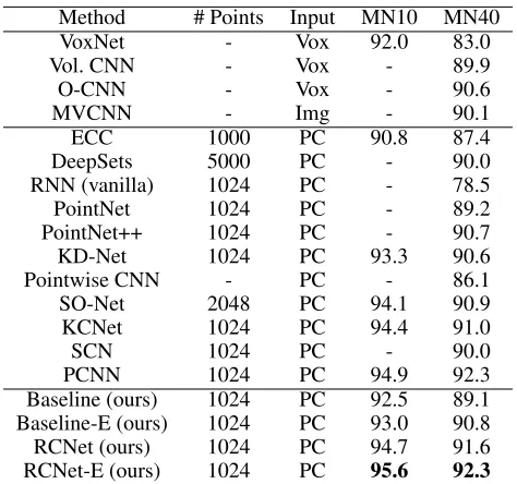
Results We compare RCNet with several state-of-the-arts: VoxNet (Maturana and Scherer 2015b), volumetric CNN (Qi et al. 2016), O-CNN (Wang et al. 2017), MVCNN (Su et al. 2015), ECC (Simonovsky and Komodakis 2017), DeepSets (Ravanbakhsh, Schneider, and Poczos 2017), vanilla RNN and PointNet (Qi et al. 2017a), PointNet++ (Qi et al. 2017b), KD-Net (Klokov and Lempitsky 2017), Pointwise CNN (Hua, Tran, and Yeung 2018), SO-Net (Li, Chen, and Lee 2018), KCNet (Shen et al. 2018), SCN (Xie et al. 2018), and PCNN (Atzmon, Maron, and Lipman 2018). The results are demonstrated in Table 1.
Method # Points Input MN10 MN40
VoxNet - Vox 92.0 83.0
Vol. CNN - Vox - 89.9
O-CNN - Vox - 90.6
MVCNN - Img - 90.1
ECC 1000 PC 90.8 87.4
DeepSets 5000 PC - 90.0 RNN (vanilla) 1024 PC - 78.5 PointNet 1024 PC - 89.2 PointNet++ 1024 PC - 90.7 KD-Net 1024 PC 93.3 90.6 Pointwise CNN - PC - 86.1 SO-Net 2048 PC 94.1 90.9 KCNet 1024 PC 94.4 91.0
SCN 1024 PC - 90.0
PCNN 1024 PC 94.9 92.3
Baseline (ours) 1024 PC 92.5 89.1 Baseline-E (ours) 1024 PC 93.0 90.8 RCNet (ours) 1024 PC 94.7 91.6 RCNet-E (ours) 1024 PC 95.6 92.3
Table 1: Classification accuracies on ModelNet datasets. (“Vox”: Voxels; “Img”: Images; “PC”: Point Clouds.)
the performance is further boosted. In particular, RCNet per-forms better than most existing approaches. While obtaining similar accuracy to PCNN, our network is significantly sim-pler in design. On the other hand, compared to the baseline model, RCNet outperforms it by a large margin. This vali-dates the effectiveness of recurrent encoder at modeling the relative relationships among points. It is worth noting that, in (Li, Chen, and Lee 2018) the SO-Net also attempted to apply the standard CNN to the generated image-like feature maps, but only led to decreased performance. In contrast, our RCNet is better at incorporating the advantages of CNN into point cloud analysis, thanks to the recurrent set encoder. Finally, our RCNet is computationally efficient. In par-ticular, a single RCNet can be trained in about 3 hours. This is much faster than PointNet++ and PCNN, both of which require about 20 hours for training (Qi et al. 2017b; Atzmon, Maron, and Lipman 2018). Besides, as shown in Table 2, on average it takes about 0.4 milliseconds for RC-Net to forward a shape, while PointRC-Net++ and PCNN re-quire 2.8 and 16.8 milliseconds, respectively1. Table 2 also
summarizes the number of parameters of different networks. Interestingly, although our model has larger size, it still runs faster than other competitors. This validates that the classic RNN and 2D CNN, which are well supported at both soft-ware and hardsoft-ware levels, contribute largely to the model ef-ficiency. In contrast, since PointNet++ need to perform ad-ditional K-nearest neighbor query on the fly on GPU, it is much less efficient in spite of the smaller model size.
Simi-1
For PCNN, we run the code released by the authors (https://github.com/matanatz/pcnn), with the default pointconv configuration. For PointNet++, we use the official implementation (https://github.com/charlesq34/pointnet2), and test the MSG model with the default network setting.
Method Infer. Time (ms) # Param. (M) Class. Seg. Class. Seg. RCNet (ours) 0.4 4.5 13.3 16.7 RCNet-E (ours) 0.6 4.8 39.9 50.1 PointNet++ 2.8 11.9 1.0 1.7
PCNN 16.8 109.3 8.1 5.4 SPLATNet3D - 23.1 - 2.7
Table 2: Comparison of inference time and model size for different networks. Classification and segmentation are per-formed on ModelNet40 and ShapeNet part datasets, respec-tively. Time is measured in milliseconds, which correspond to the cost of forwarding a shape on average. The hardware used is an Intel i7-6850K CPU and a single NVIDIA GTX 1080 Ti GPU. “M” stands for million.
larly, PCNN and SPLATNet3Drely on sophisticated
geomet-ric transformations and complex convolutional operations. These operations are much less GPU-friendly and cause a lot of overhead in practice. It is worth mentioning that, since RCNet-E is naturally parallelizable, its inference time is al-most the same with that of a single RCNet.
Shape Part Segmentation
Dataset and Configuration For shape part segmentation, the task is to classify each point of a point cloud into one of the predefined part categories. We evaluate the proposed method on the challenging ShapeNet part dataset (Yi et al. 2016), which contains 16881 shapes from 16 categories. The shapes are consistently aligned and normalized to fit within a unit ball. For each shape, it is annotated with 2-6 part labels, and in total there are 50 different parts. We sample 2048 points for each shape following (Qi et al. 2017a; 2017b). As in (Qi et al. 2017b), apart from point positions we also use normal information as input features. Following the setting in (Yi et al. 2016), we evaluate our methods assuming that the category of the input 3D shape is already known. The segmentation results are reported with the standard metric mIoU (Qi et al. 2017a). We use the official train/test split as in (Chang et al. 2015) in our experiment. We follow the same network configuration with the classification task.
Results Table 3 compares RCNet with the following state-of-the-art point cloud-based methods: PointNet (Qi et al. 2017a), PointNet++ (Qi et al. 2017b), Kd-Net (Klokov and Lempitsky 2017), SPLATNet3D (Su et al. 2018), SO-Net
(pre-trained) (Li, Chen, and Lee 2018), RSNet (Huang, Wang, and Neumann 2018), KCNet (Shen et al. 2018), A-SCN (Xie et al. 2018), and PCNN (Atzmon, Maron, and Lipman 2018). In Table 3, we report the instance average mIoU as well as the mIoU scores for each category.
mean aero bag cap car chair ear-p guitar knife lamp laptop motor mug pistol rocket skate table
# shapes 2690 76 55 898 3758 69 787 392 1547 451 202 184 283 66 152 5271
PointNet 83.7 83.4 78.7 82.5 74.9 89.6 73.0 91.5 85.9 80.8 95.3 65.2 93.0 81.2 57.9 72.8 80.6 PointNet++ 85.1 82.4 79.0 87.7 77.3 90.8 71.8 91.0 85.9 83.7 95.3 71.6 94.1 81.3 58.7 76.4 82.6 Kd-Net 82.3 80.1 74.6 74.3 70.3 88.6 73.5 90.2 87.2 81.0 94.9 57.4 86.7 78.1 51.8 69.9 80.3 SPLATNet3D 84.6 81.9 83.9 88.6 79.5 90.1 73.5 91.3 84.7 84.5 96.3 69.7 95.0 81.7 59.2 70.4 81.3 SO-Net (p.t.) 84.9 82.8 77.8 88.0 77.3 90.6 73.5 90.7 83.9 82.8 94.8 69.1 94.2 80.9 53.1 72.9 83.0 RSNet 84.9 82.7 86.4 84.1 78.2 90.4 69.3 91.4 87.0 83.5 95.4 66.0 92.6 81.8 56.1 75.8 82.2 KCNet 84.7 82.8 81.5 86.4 77.6 90.3 76.8 91.0 87.2 84.5 95.5 69.2 94.4 81.6 60.1 75.2 81.3 A-SCN 84.6 83.8 80.8 83.5 79.3 90.5 69.8 91.7 86.5 82.9 96.0 69.2 93.8 82.5 62.9 74.4 80.8 PCNN 85.1 82.4 80.1 85.5 79.5 90.8 73.2 91.3 86.0 85.0 95.7 73.2 94.8 83.3 51.0 75.0 81.8 Baseline (ours) 84.6 83.3 76.8 87.6 78.6 90.3 73.7 90.9 86.8 82.1 95.5 69.8 94.3 82.6 58.4 76.0 81.7 Baseline-E (ours) 85.3 84.1 77.0 87.4 79.8 90.6 73.9 91.5 87.0 83.1 95.6 70.0 94.4 83.4 58.1 75.6 82.4 RCNet (ours) 85.3 84.4 80.1 89.6 78.6 90.5 76.3 91.4 87.3 82.5 96.1 73.1 94.7 84.0 61.0 76.1 82.6 RCNet-E (ours) 86.0 85.3 81.1 90.0 79.9 91.1 77.0 91.8 87.3 84.1 96.5 75.1 95.1 84.8 61.3 76.4 83.1
Table 3: Results on ShapeNet part segmentation. mIoU metric is used for evaluation. The instance average mIoU as well as mIoU scores for each shape category are listed. Our RCNet-E outperforms the state-of-the-arts in most categories and achieves the best instance average mIoU.
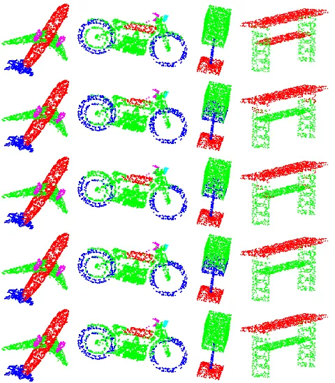
Figure 2: Visualization of ShapeNet part segmentation re-sults. From top to bottom: ground truth, baseline, baseline-E, RCNet, RCNet-E. From left to right: airplane, motorbike, lamp, table.
two columns show that both RCNet and RCNet-E are able to handle the small details of objects well. The third col-umn indicates that the ensemble helps correct the prediction error of a single model, and is better at capturing the fine-grain semantics than the baseline methods. The last column corresponds to a failure case, which is possibly due to the imperfect model representation ability or caused by shape semantic ambiguity (i.e., the table board in the middle could be interpreted as either table support or tabletop).
Method Mean IoU Overall accuracy PointNet 47.71 78.62
A-SCN 52.72 81.59
Pointwise CNN - 81.50 Baseline (ours) 50.31 81.57 Baseline-E (ours) 52.38 82.98 RCNet (ours) 51.40 82.01 RCNet-E (ours) 53.21 83.58
Table 4: Segmentation results on S3DIS dataset. Mean IoU and point-wise accuracy are listed.
In Table 2, we compare the computational efficiency of different networks on part segmentation task. As is shown, our method is more efficient than the state-of-the-arts2.
Semantic Scene Segmentation
Dataset and Configuration We evaluate our RCNet on the scene parsing task with Standford 3D indoor scene dataset (S3DIS) (Armeni et al. 2016). S3DIS consists of 6 scanned large-scale areas, which in total have 271 rooms. Each point in the scene point cloud is annotated with one of the 13 semantic categories. Following (Qi et al. 2017a), we pre-process the data by splitting the scene points into rooms, and then subdividing the rooms into small blocks with area 1m by 1m (measured on the floor). As in (Qi et al. 2017a), we also use k-fold strategy for training and testing. At train-ing time we randomly sample 2048 points for each block, but use all the points during testing. We represent each point using 9 attributes, including XYZ coordinates, RGB values and normalized coordinates as to the room. The same shape segmentation RCNet is used for this task.
Results We compare our RCNet with PointNet (Qi et al. 2017a), A-SCN (Xie et al. 2018) and Pointwise CNN (Hua,
2
For SPLATNet3D, we run the code implemented by the
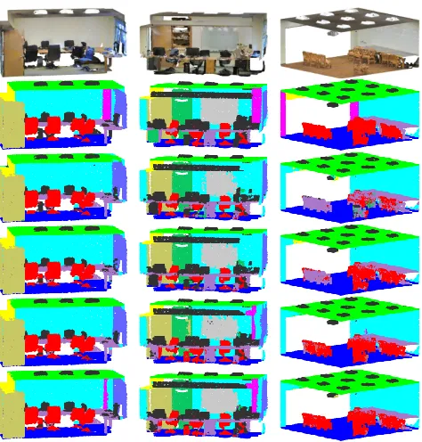
Figure 3: Visualization of S3DIS segmentation results. From top to bottom: input scene, ground truth, baseline, baseline-E, RCNet, RCNet-E.
Tran, and Yeung 2018). The results are reported in Table 4. As is shown, our RCNet improves A-SCN by about0.5%in mean IoU and2% in overall accuracy. We visualize a few segmentation results in Fig. 3. It can be observed that RC-Net is able to output smooth predictions and segment the small objects well. In contrast, the baseline methods tend to produce large prediction errors. This shows the benefits of our recurrent set encoder and the 2D CNN as feature aggre-gators. With ensemble, the segmentation accuracy is further boosted and our RCNet-E achieves the best results.
Architecture Analysis
In this section we show the effects of network hyper-parameters and validate the design choices through a se-ries of controlled experiments. We consider the following two main contributory factors on model performance: (1) the size of beams; (2) the number of points. We use ModelNet40 dataset as the test bed for comparisons of different options. Unless explicitly noted, all the experimental settings are the same with those in the shape classification experiment.
The Size of Beams The beam size controls how much lo-cal context information would be utilized, and is a major contributory factor for the network performance. For RC-Net, large beams will lead to a small feature map for the downstream CNN. This would increase the efficiency of CNN but in turn result in the loss of fine-scale geometric de-tails. Moreover, beams with large size would be filled with too many points, and as a result the RNN would perform poorly in feature modeling. On the other hand, if the size of beams is too small, the subregions would contain insufficient
r×s 8×8 16×16 32×32 64×64 128×128
Baseline 77.2 86.3 89.1 89.3 86.7 RCNet 87.5 90.2 91.6 90.9 89.8
Table 5: The influence of beam size on network perfor-mance. The smaller the hyper-parametersrands, the larger the beams, and vice versa. The experiments are conducted on ModelNet40, and the metric is classification accuracy.
# Point Baseline + DP RCNet + DP Baseline RCNet
1024 88.9 91.1 88.2 90.2
512 88.2 90.4 68.2 76.2
256 87.7 90.2 35.3 38.1
128 86.4 87.8 17.8 24.9
Table 6: Experiments on robustness to non-uniform and sparse data. DP stands for random point dropout during training. The experiments are conducted on ModelNet40.
amount of points, which is adverse to the feature learning. We conduct several experiments to investigate the influ-ence of beam size on the network performance. In partic-ular, we test RCNet with different specifications of hyper-parametersrands. The results are reported in Table 5. As is shown, both larger and smaller beam sizes would hurt the performance, and r×s = 32×32leads to the best re-sults. Note that, although beam size is an important param-eter on the performance, our RCNet is still quite robust to this factor. In contrast, the max-pooling based encoder be-haves quite sensitively and the performance decreases a lot with large beams. This further validates that pooling is a rel-atively coarse technique for exploiting geometric details.
The Number of Points Point clouds obtained from sen-sors in real world usually suffer from data corruptions, which lead to non-uniform data with varying densities (Qi et al. 2017b). To validate the robustness of our model to such situations, we randomly dropout the number of points in testing and conduct two different groups of experiments. In the first group, the models are trained on uniform point clouds without random point dropout, while in the second group the models are trained with random dropout as well. In the experiment, we setr=s= 32as in the shape classi-fication task. The results are shown in Table 6. We observe that models trained with random point dropout (DP) during training are fairly robust to the sampling density variation, with drop of accuracy less than 3.3% when point number decreases from 1024 to 128. In contrast, those trained only on uniform data fail to generalize well to the cases of non-uniform data. Note that, despite the drop of accuracy, our RCNet still achieves better performance than the baseline model when trained without DP. This validates the superi-ority of RNN in subregional feature extraction compared to max-pooling.
Conclusion and Discussion
set encoder and a 2D CNN. The recurrent set encoder parti-tions the input point clouds into several parts, which are en-coded via a shared RNN. The enen-coded part features are later assembled in a structured manner and fed into a 2D CNN for global feature learning. Such design leads to an efficient as well as effective network, thanks to the benefits of CNN and RNN. Experiments on four representative datasets show that our method competes favorably with the state-of-the-arts in terms of accuracy and efficiency. We also conduct extensive experiments to further analyze the network properties, and show that our method is quite robust to several key factors affecting the model performance.
Finally, we note that the proposed recurrent set encoder can be generalized to other contexts. For example, we can build a KNN graph for the input point cloud and model the local neighborhood for each point with recurrent encoder. In particular, we can sort theknearest neighbor points ac-cording to their distances to the query point, and then apply RNN to this point sequence for local feature learning. This is different from KCNet (Shen et al. 2018) which uses a local point-set kernel, and will be explored in the future.
Acknowledgments
This work was partially supported by NSF IIS-1718802, CCF-1733866, and CCF-1733843.
References
Armeni, I.; Sener, O.; Zamir, A. R.; Jiang, H.; Brilakis, I.; Fischer, M.; and Savarese, S. 2016. 3d semantic parsing of large-scale indoor spaces. InIEEE Conference on Computer Vision and Pattern Recognition (CVPR), 1534–1543.
Atzmon, M.; Maron, H.; and Lipman, Y. 2018. Point con-volutional neural networks by extension operators. InACM SIGGRAPH.
Boscaini, D.; Masci, J.; Melzi, S.; Bronstein, M. M.; Castel-lani, U.; and Vandergheynst, P. 2015. Learning class-specific descriptors for deformable shapes using localized spectral convolutional networks. Comput. Graph. Forum34(5):13– 23.
Bronstein, M. M.; Bruna, J.; LeCun, Y.; Szlam, A.; and Van-dergheynst, P. 2017. Geometric deep learning: Going be-yond euclidean data. IEEE Signal Process. Mag.34(4):18– 42.
Bruna, J.; Zaremba, W.; Szlam, A.; and LeCun, Y. 2014. Spectral networks and locally connected networks on graphs. InInternational Conference on Learning Represen-tations (ICLR).
Chang, A. X.; Funkhouser, T. A.; Guibas, L. J.; Hanrahan, P.; Huang, Q.; Li, Z.; Savarese, S.; Savva, M.; Song, S.; Su, H.; Xiao, J.; Yi, L.; and Yu, F. 2015. Shapenet: An information-rich 3d model repository.CoRRabs/1512.03012.
Chen, X.; Ma, H.; Wan, J.; Li, B.; and Xia, T. 2017. Multi-view 3d object detection network for autonomous driving. In
IEEE Conference on Computer Vision and Pattern Recogni-tion (CVPR), 6526–6534.
Chung, J.; G¨ulc¸ehre, C¸ .; Cho, K.; and Bengio, Y. 2014. Em-pirical evaluation of gated recurrent neural networks on se-quence modeling. InNIPS Workshop on Deep Learning. Defferrard, M.; Bresson, X.; and Vandergheynst, P. 2016. Convolutional neural networks on graphs with fast localized spectral filtering. In Advances in Neural Information Pro-cessing Systems (NIPS), 3837–3845.
Hua, B.-S.; Tran, M.-K.; and Yeung, S.-K. 2018. Point-wise convolutional neural networks. In IEEE Conference on Computer Vision and Pattern Recognition (CVPR), 984– 993.
Huang, Q.; Wang, W.; and Neumann, U. 2018. Recur-rent slice networks for 3d segmentation of point clouds. In
IEEE Conference on Computer Vision and Pattern Recogni-tion (CVPR), 2626–2635.
Jaderberg, M.; Simonyan, K.; Zisserman, A.; and Kavukcuoglu, K. 2015. Spatial transformer networks. In Advances in Neural Information Processing Systems (NIPS), 2017–2025.
Kalogerakis, E.; Averkiou, M.; Maji, S.; and Chaudhuri, S. 2017. 3d shape segmentation with projective convolutional networks. InIEEE Conference on Computer Vision and Pat-tern Recognition (CVPR), 6630–6639.
Kehoe, B.; Patil, S.; Abbeel, P.; and Goldberg, K. 2015. A survey of research on cloud robotics and automation. IEEE Trans. Automation Science and Engineering12(2):398–409. Kingma, D. P., and Ba, J. 2015. Adam: A method for stochastic optimization. In International Conference on Learning Representations (ICLR).
Kipf, T. N., and Welling, M. 2017. Semi-supervised classi-fication with graph convolutional networks. InInternational Conference on Learning Representations (ICLR).
Klokov, R., and Lempitsky, V. S. 2017. Escape from cells: Deep kd-networks for the recognition of 3d point cloud models. InIEEE International Conference on Computer Vi-sion (ICCV), 863–872.
Li, R.; Wang, S.; Zhu, F.; and Huang, J. 2018. Adaptive graph convolutional neural networks. InAAAI.
Li, J.; Chen, B. M.; and Lee, G. H. 2018. So-net: Self-organizing network for point cloud analysis. In IEEE Conference on Computer Vision and Pattern Recognition (CVPR).
Liu, F.; Li, S.; Zhang, L.; Zhou, C.; Ye, R.; Wang, Y.; and Lu, J. 2017. 3dcnn-dqn-rnn: A deep reinforcement learn-ing framework for semantic parslearn-ing of large-scale 3d point clouds. InIEEE International Conference on Computer Vi-sion (ICCV), 5679–5688.
Liu, M. 2016. Robotic online path planning on point cloud.
IEEE Trans. Cybernetics46(5):1217–1228.
Maturana, D., and Scherer, S. 2015a. 3d convolutional neural networks for landing zone detection from lidar. In
IEEE International Conference on Robotics and Automation (ICRA), 3471–3478.
InIEEE/RSJ International Conference on Intelligent Robots and Systems (IROS), 922–928.
Qi, C. R.; Su, H.; Nießner, M.; Dai, A.; Yan, M.; and Guibas, L. J. 2016. Volumetric and multi-view cnns for object classi-fication on 3d data. InIEEE Conference on Computer Vision and Pattern Recognition (CVPR), 5648–5656.
Qi, C. R.; Su, H.; Mo, K.; and Guibas, L. J. 2017a. Pointnet: Deep learning on point sets for 3d classification and segmen-tation. InIEEE Conference on Computer Vision and Pattern Recognition (CVPR), 77–85.
Qi, C. R.; Yi, L.; Su, H.; and Guibas, L. J. 2017b. Point-net++: Deep hierarchical feature learning on point sets in a metric space. InAdvances in Neural Information Processing Systems (NIPS), 5105–5114.
Ravanbakhsh, S.; Schneider, J.; and Poczos, B. 2017. Deep learning with sets and point clouds. InInternational Confer-ence on Learning Representations Workshop (ICLRW). Riegler, G.; Ulusoy, A. O.; and Geiger, A. 2017. Octnet: Learning deep 3d representations at high resolutions. In
IEEE Conference on Computer Vision and Pattern Recog-nition (CVPR), 6620–6629.
Sedaghat, N.; Zolfaghari, M.; and Brox, T. 2017. Orientation-boosted voxel nets for 3d object recognition. In
British Machine Vision Conference (BMVC).
Shen, Y.; Feng, C.; Yang, Y.; and Tian, D. 2018. Mining point cloud local structures by kernel correlation and graph pooling. InIEEE Conference on Computer Vision and Pat-tern Recognition (CVPR).
Simonovsky, M., and Komodakis, N. 2017. Dynamic edgeconditioned filters in convolutional neural networks on graphs. InIEEE Conference on Computer Vision and Pat-tern Recognition (CVPR).
Su, H.; Maji, S.; Kalogerakis, E.; and Learned-Miller, E. G. 2015. Multi-view convolutional neural networks for 3d shape recognition. In IEEE International Conference on Computer Vision (ICCV), 945–953.
Su, H.; Jampani, V.; Sun, D.; Maji, S.; Kalogerakis, E.; Yang, M.; and Kautz, J. 2018. Splatnet: Sparse lattice net-works for point cloud processing. InIEEE Conference on Computer Vision and Pattern Recognition (CVPR).
Tatarchenko, M.; Dosovitskiy, A.; and Brox, T. 2017. Oc-tree generating networks: Efficient convolutional architec-tures for high-resolution 3d outputs. InIEEE International Conference on Computer Vision (ICCV), 2107–2115. Tchapmi, L. P.; Choy, C. B.; Armeni, I.; Gwak, J.; and Savarese, S. 2017. Segcloud: Semantic segmentation of 3d point clouds. InInternational Conference on 3D Vision (3DV).
Vinyals, O.; Bengio, S.; and Kudlur, M. 2016. Order mat-ters: Sequence to sequence for sets. InInternational Confer-ence on Learning Representations (ICLR).
Wang, P.; Liu, Y.; Guo, Y.; Sun, C.; and Tong, X. 2017. O-CNN: octree-based convolutional neural networks for 3d shape analysis.ACM Trans. Graph.36(4):72:1–72:11. Wang, S.; Suo, S.; Ma, W.-C.; Pokrovsky, A.; and Urtasun,
R. 2018. Deep parametric continuous convolutional neu-ral networks. InIEEE Conference on Computer Vision and Pattern Recognition (CVPR), 2589–2597.
Wu, Z.; Song, S.; Khosla, A.; Yu, F.; Zhang, L.; Tang, X.; and Xiao, J. 2015. 3d shapenets: A deep representation for volumetric shapes. InIEEE Conference on Computer Vision and Pattern Recognition (CVPR), 1912–1920.
Xie, S.; Liu, S.; Chen, Z.; and Tu, Z. 2018. Atten-tional shapecontextnet for point cloud recognition. InIEEE Conference on Computer Vision and Pattern Recognition (CVPR).